October 17, 2026

What this problem really is

Leverage is often presented as a simple multiplier: a trader puts down a fraction of the notional, the broker supplies the rest, and the resulting position is said to be “5×” or “10×”. The reality is far richer. When a market moves against a leveraged book, the loss is not merely a function of the volatility that was observed yesterday; it is a function of the depth of the order book, the speed at which margin calls can be met, and the correlation of the positions that generate the exposure. In practice the gross notional that a desk holds can be many times larger than the capital that would be exhausted by a modest adverse price swing. The distinction between gross exposure and capital at risk is the first line of defence against a cascade of losses that can be triggered by a single, seemingly innocuous price move.

If the desk treats the maximum permitted margin as the only sizing constraint, it implicitly assumes that the market will always provide sufficient liquidity to unwind or hedge the position at the quoted spread. That assumption collapses the moment a stress gap appears, spreads widen, or a margin requirement is revised. The resulting “account risk” is not a theoretical construct; it is the capital that must be liquidated or replenished under duress, and it can be far larger than the nominal margin figure suggests.

How the mechanism works, step by step

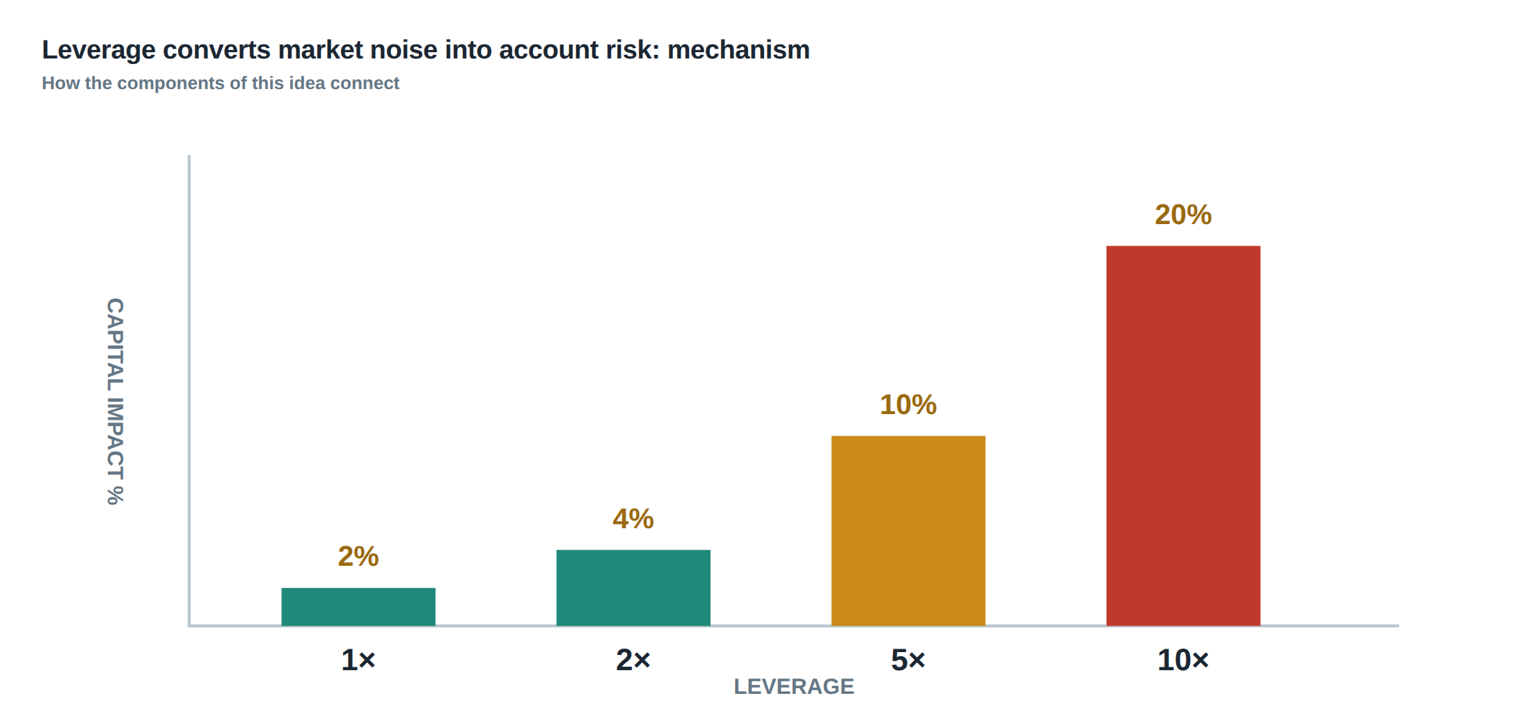
The first step is to separate the gross exposure of each strategy from the capital that would be lost if the exposure were to be liquidated at the worst plausible price. Gross exposure is simply the notional of all open positions, irrespective of direction. Capital at risk is derived by applying a stress scenario – for example a 2 % move in the underlying – to the net exposure after accounting for the current spread, the expected execution cost, and any hedging that can be performed with available cash.

Second, the desk must model the liquidity required to meet variation margin calls and to execute emergency hedges. This involves estimating the size of the order book that can be accessed without moving the price beyond the stress move, and the time it would take to traverse that depth. If the required cash cannot be generated within the margin call window, the position will be forced into a forced‑sale regime, which typically incurs a further spread widening.

Third, the aggregation of leverage across correlated positions must be performed. Two ostensibly independent strategies may share exposure to the same underlying risk factor; their individual leverage numbers are therefore misleading if summed without correlation adjustment. The aggregate leverage is the ratio of the combined stressed loss to the total capital, and it will often be higher than any single strategy’s leverage because the stress scenarios are applied to the net of the correlated exposures.

A worked example with real numbers

Consider a prop‑desk that allocates £1 million of capital to a high‑frequency statistical arbitrage strategy. The desk decides to run the strategy at five times gross exposure, meaning the notional of all open positions is £5 million. The typical daily volatility of the underlying basket is 1 %, and the average spread cost is 0.05 % of notional. Under normal conditions a 2 % adverse move would be considered a tail event, but the desk treats it as the plausible worst‑case for sizing purposes.

A 2 % move on a £5 million exposure translates to a £100 000 mark‑to‑market loss. Adding the spread cost of £2 500 (0.05 % of £5 million) brings the total to £102 500. Because the strategy is leveraged five times, the loss represents roughly ten percent of the original £1 million capital. In other words, a price swing that is only twice the typical daily volatility can erode a tenth of the desk’s equity before any additional costs such as slippage, forced‑sale discounts, or margin calls are taken into account.

If the desk had instead sized the exposure based on the maximum permitted margin – say a 20 % utilisation of the capital – it would have allowed a gross exposure of £5 million without recognising that a modest 2 % move already threatens a substantial fraction of the capital. The example demonstrates that leverage converts ordinary market noise into a material account‑risk event when the sizing discipline is anchored to margin limits rather than to stress‑adjusted liquidity.

Where it breaks in live markets

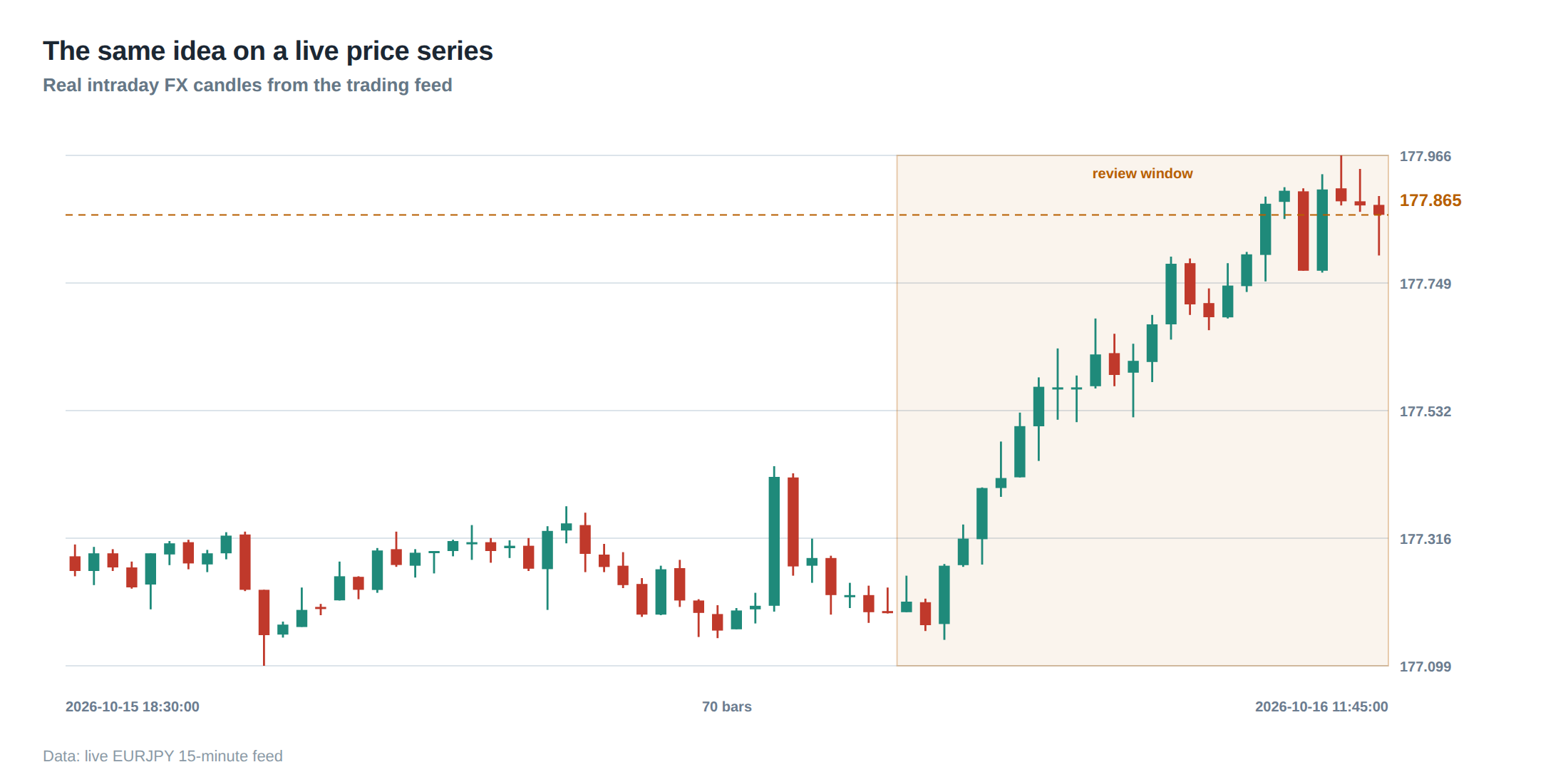
The theoretical framework collapses the moment market microstructure deviates from the assumptions used in the stress model. Gaps can appear in the order book when a large hidden order is withdrawn, when a news event triggers a rapid reassessment of valuation, or when a venue experiences a temporary outage. In those moments the spread can expand from a few basis points to several dozen, and the price required to execute a hedge may be far beyond the 2 % stress move used in the example.

Margin requirements are not static. Regulatory or clearing‑house policy can change overnight, increasing the initial margin by a factor of two or more. When such a change occurs, the cash that was earmarked for variation margin may be insufficient, forcing the desk to liquidate positions at a price that already reflects the widened spread. The resulting feedback loop amplifies the initial loss, turning a manageable stress scenario into a capital‑draining event.

The research that underpins modern risk analysis stresses the importance of looking beyond the mean or median of a return distribution. It shows that a single realised outcome cannot capture the tail risk inherent in fast‑moving strategies. In practice this means that latency statistics, average fill quality, and typical order‑book depth are inadequate; the tail of the latency distribution, the frequency of stale orders, and the loss profile when routing behaves abnormally must be incorporated into the risk model.

The operating path, stage by stage

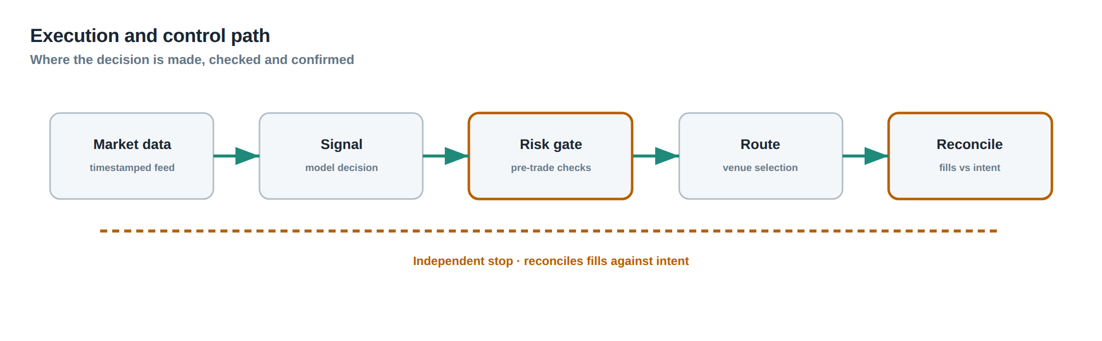
Stage one is the pre‑trade liquidity assessment. The trader queries the depth of the market at the intended price level, applies a discount for expected slippage, and records the cash required to cover the worst‑case spread expansion. Stage two is the capital allocation engine, which takes the stress‑adjusted cash requirement and compares it to the available liquidity buffer, not to the contractual margin limit. If the buffer is insufficient, the trade is either reduced in size or rejected outright.

Stage three is the real‑time monitoring loop. As the market evolves, the system continuously recomputes the stress loss based on the latest order‑book snapshot, and it watches for any breach of the pre‑defined liquidity threshold. When a breach is imminent, an automated hedge is triggered, drawing on the reserved cash. Stage four is the post‑trade reconciliation, where the realised P&L is compared to the stress scenario to validate the assumptions used in the pre‑trade model.

Each stage must be documented, auditable, and subject to independent verification. The flow of information from market data feeds to the capital allocation module and finally to the execution engine must be lossless; any data latency or corruption can cause the stress model to underestimate the true exposure at the moment of execution.

Controls that act before the damage

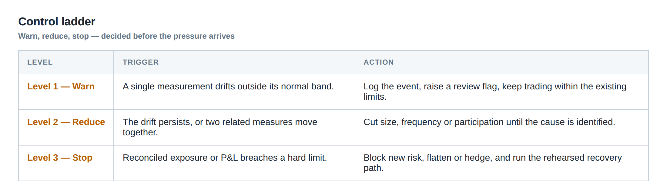
The first line of defence is a hard stop on aggregate leverage that is computed after correlation adjustment. The stop is enforced at the capital‑allocation layer, preventing the sum of stressed losses from exceeding a pre‑agreed fraction of the total equity, typically no more than 15 % for high‑frequency strategies. The second control is a dynamic liquidity reserve that is sized each day based on the worst‑case spread and gap scenarios identified in the pre‑trade assessment. This reserve sits in cash or highly liquid assets that can be deployed instantly to meet variation margin or to fund emergency hedges.

A third control is the mandatory stress‑test run on every new instrument or strategy before it is permitted to trade. The test runs a battery of scenarios – including rapid price jumps, order‑book depletion, and margin‑requirement spikes – and records the capital at risk under each. If any scenario breaches the capital‑at‑risk threshold, the strategy is either re‑parameterised or barred.

The final control is a real‑time alerting system that flags when the live spread deviates from the modelled spread by more than a predefined multiple of the historical standard deviation. When the alert fires, the execution engine automatically throttles order flow or switches to a more liquid venue, thereby limiting the exposure to an expanding spread.

How to measure whether it is working

Effectiveness is measured by comparing the realised loss distribution against the stress‑adjusted loss distribution that was used for sizing. The key metric is the exceedance ratio: the proportion of trading days on which the realised loss exceeds the pre‑trade stress loss. A well‑tuned system should keep this ratio below the confidence level used in the stress model, typically 5 %.

Another indicator is the utilisation of the liquidity reserve. If the reserve is consistently drawn down and not replenished, the sizing framework is too aggressive. Conversely, a reserve that never moves suggests that the stress assumptions are overly conservative and capital is being under‑utilised.

A third measurement is the correlation‑adjusted aggregate leverage over time. By plotting this metric against the capital‑at‑risk threshold, the desk can see whether leverage spikes coincide with market stress events. A stable gap indicates that the aggregation control is functioning; frequent breaches point to hidden correlations or mis‑estimated stress scenarios.

The portfolio view

When the desk looks at the portfolio as a whole, the individual stress‑adjusted exposures must be summed with their correlation matrix to obtain the true capital at risk. This aggregate figure replaces the naïve sum of gross notionals that many desks still use for reporting. The portfolio‑level leverage, defined as the ratio of total stressed loss to total equity, provides a single, comparable number across strategies and asset classes.

Because each strategy contributes to the liquidity reserve, the portfolio view also includes the net cash buffer after accounting for the reserve requirements of all constituent strategies. The buffer is then allocated proportionally to the marginal contribution of each strategy to the aggregate leverage. This ensures that a strategy that adds the most to portfolio‑level risk also carries the largest share of the liquidity safety net.

In practice, the portfolio view is refreshed at the end of each trading day, and any breach of the aggregate leverage threshold triggers a rebalancing of notional limits across the desk. The rebalancing respects the hierarchy of risk appetite – for example, market‑making desks may be given a higher tolerance than pure directional bets – but always within the envelope defined by the stress‑adjusted capital at risk.

Do you currently size your positions based on a stress‑adjusted liquidity analysis, or do you still rely on the maximum permitted margin as the primary constraint?

About the research behind this lesson

Andrew Lo's lectures build risk analysis from return distributions and statistical measures, rather than treating one realised result as a complete description of risk.

Applied to this lesson: For a fast strategy, median latency or average fill quality is not enough. The review has to include tail delays, stale-order frequency and the loss distribution when cancellation or routing behaves abnormally.

Explore PULSE: System details

PULSE live account: Verify the live account on FX Blue

Live chat and updates: Telegram @xtrskhft

Source: Risk and Return

Educational content only. Trading leveraged products involves risk.