November 5, 2026

What this problem really is

In a modern electronic market every incoming quote is a time‑sensitive contract between a trading algorithm and the venue’s matching engine. The moment a signal is generated, a decision is made to place an order, but the order does not appear instantaneously at the top of the book. It first traverses a local gateway, then a network link, then the exchange’s inbound queue, before finally being admitted to the price‑time priority line. During each of those stages the market can move, the spread can narrow, and the statistical edge that justified the signal can evaporate. Consequently the “lifetime” of a signal is not simply the wall‑clock time elapsed since the signal fired; it is the interval during which the order’s expected value remains positive given its current queue position and the prevailing adverse‑selection risk. If the order remains in the system after that interval, the original signal has become stale, yet the order may still be executed or sit in the book, exposing the desk to unintended risk.

The problem is compounded when a cancellation is required. A local cancel request is generated instantly, but the acknowledgement that the venue has removed the order from its queue can be delayed by milliseconds to seconds, especially under high load or when the order sits deep in the queue. Until the confirmation arrives the order is still “alive” in the market’s eyes, and any subsequent price move may be captured against a position that the strategy no longer wishes to hold. The mismatch between signal expiry and order existence creates a hidden exposure that can turn a theoretically risk‑free micro‑arb into a loss.

How the mechanism works, step by step

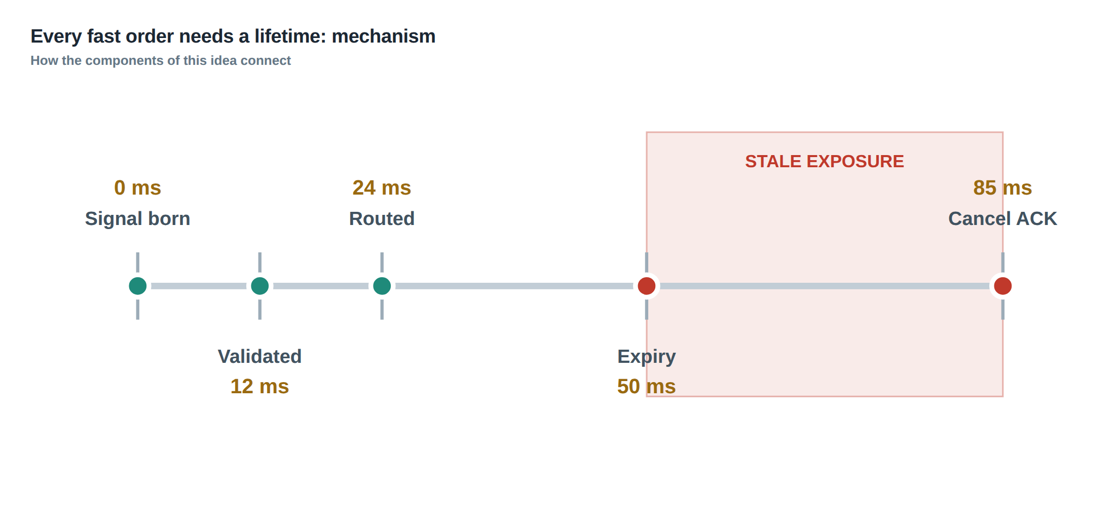
The first step is the generation of a trading signal. The signal is evaluated against a pre‑defined maximum age – for example, a 50 ms window for a micro‑price‑dislocation strategy. If the signal is still valid after that window, the algorithm proceeds to create a new order packet. The packet is timestamped and handed to the local order‑management system (OMS), which appends a unique client order identifier and a “time‑to‑live” (TTL) field equal to the remaining signal age.

The OMS then forwards the packet to the network stack. At this point the order is subject to latency jitter, which can be measured by round‑trip time (RTT) probes. Once the packet reaches the exchange gateway, the venue timestamps the receipt and places the order into its inbound queue. The exchange assigns a sequence number that determines the order’s position in the price‑time priority line. If the order is a limit order inside the spread, it will sit waiting for a matching taker; if it is a marketable order, it will be executed immediately but still carries the risk that the execution price is now unfavourable relative to the original signal.

When market conditions change such that the signal is no longer profitable, the OMS issues a cancel request. The local system marks the order as “cancellation pending” and records the request timestamp. The request follows the same network path back to the venue, where it is queued behind any inbound traffic. Only after the exchange processes the cancel does it emit a cancellation acknowledgement (ACK). Until that ACK is received, the order remains in the venue’s queue and can still be matched. The algorithm must therefore treat the interval between local request and venue ACK as a “danger window” and decide whether to let the order sit, replace it, or abort further exposure through other controls.

A worked example with real numbers

Consider a strategy that exploits a fleeting 0.2 % spread compression on a liquid equity futures contract. The model predicts that a 50 ms window captures the majority of the expected profit, which amounts to a theoretical 0.15 % per trade after transaction costs. At 09:30:12.345 UTC the signal fires, and the OMS creates a limit order to buy 100 contracts at the current best ask of 12 500.00. The order packet is stamped 09:30:12.345 UTC and the TTL is set to 50 ms, meaning the order should be withdrawn no later than 09:30:12.395 UTC if the spread does not widen.

The network latency from the OMS to the exchange averages 2 ms, but on this occasion a temporary congestion adds 3 ms, so the order reaches the venue at 09:30:12.350 UTC. The exchange timestamps the receipt and places the order at position 12 in the queue, because twelve other orders arrived milliseconds earlier. By the time the order reaches the front of the queue, the market has moved: the ask has risen to 12 500.30, eroding the expected profit to zero. The algorithm recognises the signal is now invalid at 09:30:12.380 UTC and issues a cancel request.

The cancel request leaves the OMS at 09:30:12.381 UTC, traverses the same 5 ms congested path, and arrives at the exchange at 09:30:12.386 UTC. However, the exchange is still processing the original order’s placement and the subsequent ten orders ahead of it, so the cancel sits in the inbound queue for another 12 ms. The venue finally emits an ACK at 09:30:12.398 UTC, after the original TTL has expired. In the interim the order has been partially filled for 30 contracts at 12 500.30, locking in a loss of 0.24 % on those contracts because the original signal’s edge has vanished. The remaining 70 contracts are cancelled, but the damage – the realised loss – has already occurred.

This example illustrates that a 50 ms signal can leave an order “alive” for 53 ms, and that a cancel acknowledgement delayed by 12 ms can turn a theoretical zero‑risk trade into a realised loss. The key numbers – 50 ms signal window, 5 ms network jitter, 12 ms cancel‑ACK delay, 30 contracts filled – are the concrete metrics that any robust system must monitor and bound.

Where it breaks in live markets

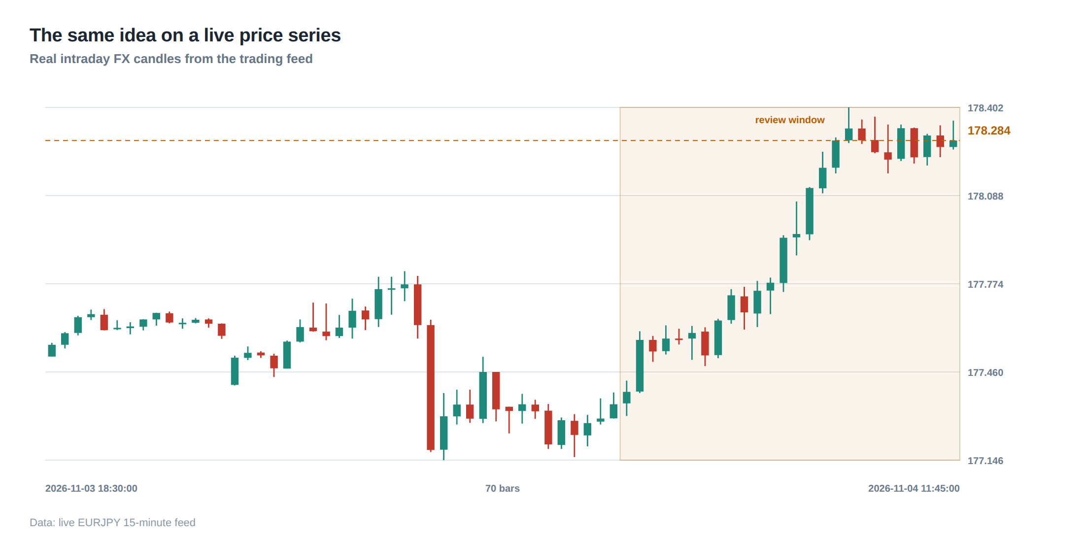
In production environments the idealised timings described above are frequently breached. During market‑open spikes, the inbound queue at the exchange can swell to thousands of orders, inflating the time required for a cancel request to be processed. Network paths that are otherwise sub‑millisecond can suffer micro‑bursts of congestion, especially when co‑located servers share the same switch fabric. Moreover, the venue’s own throttling mechanisms – such as order‑rate limits and “burst‑cancel” policies – can deliberately delay or reject cancel requests that exceed a configured threshold, turning a well‑intentioned risk‑mitigation action into a source of exposure.

Another failure mode is the “replacement storm”. When a signal’s edge decays, many strategies attempt to amend the original order with a tighter price or a smaller size. If the venue processes those amendments sequentially, each amendment must be acknowledged before the next is sent. Under high load the acknowledgements can lag, leaving a cascade of pending amendments in the system. The original order may therefore remain at an unfavourable price for longer than any individual amendment’s TTL, creating a window where the market can move against the strategy.

Finally, the separation between local and venue state is often hidden from the trader’s monitoring tools. A local OMS may report an order as “cancelled” the instant the request is issued, while the exchange still holds the order in its book. Without a mechanism to reconcile the two states, the desk may mistakenly believe that exposure has been eliminated, when in fact the order continues to sit in the queue, ready to be executed on the next matching event.

The operating path, stage by stage

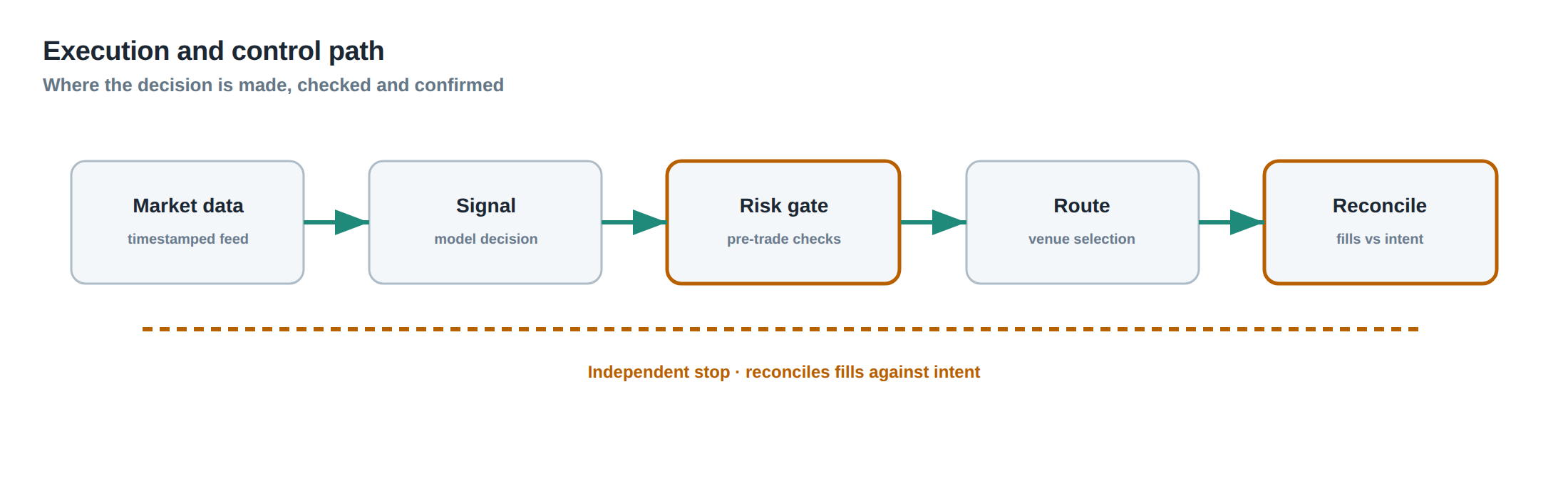
The full lifecycle can be decomposed into five distinct stages: signal generation, order creation, venue admission, active queue residence, and termination (either execution or cancellation). At the signal‑generation stage the algorithm timestamps the event and attaches a maximum‑age parameter. During order creation the OMS records the client‑side timestamp and embeds the TTL in the order’s metadata. In the venue‑admission stage the exchange’s gateway stamps the inbound packet with a receipt time and assigns a sequence number that determines queue position. While the order resides in the active queue, the system must continuously recompute the expected profit based on the current spread, depth, and adverse‑selection probability; this recomputation is the “queue‑value” assessment. The termination stage is triggered either by a fill, a venue‑confirmed cancel, or by the expiry of the TTL, at which point the OMS must decide whether to let the order sit, replace it, or issue a forced cancel.

Each stage has a measurable latency component: signal‑to‑order (algorithm processing), order‑to‑gateway (network outbound), gateway‑to‑exchange (network inbound), exchange‑queue‑wait (order‑position dependent), and cancel‑ACK (network round‑trip plus exchange processing). By instrumenting each component with high‑resolution timestamps, the desk can build a latency distribution for each stage and compare it against the signal’s maximum age. When any component’s tail exceeds a pre‑defined percentile (for example, the 99th percentile of the 50 ms window), the system should automatically flag the order for early termination.

Controls that act before the damage

A robust defence against stale‑order exposure starts with a “lifetime guard” embedded in the OMS. The guard monitors the elapsed time since the signal timestamp and, as soon as the remaining TTL falls below the worst‑case network‑plus‑exchange latency estimate, it pre‑emptively issues a cancel request with the highest possible priority flag (e.g., “immediate‑or‑cancel”). The guard also distinguishes between a local cancel request – a flag that the OMS has marked the order as “cancelling” – and a venue‑confirmed cancellation, which is only set after receipt of the ACK. Until the ACK arrives, the guard treats the order as still active and may apply a “stop‑loss” rule based on real‑time market moves, such as aborting any further exposure if the price moves more than a predefined number of ticks away from the original entry level.

Another control is the “replacement‑storm limiter”. When the algorithm detects that the signal’s edge is decaying, it caps the number of amendment attempts per unit time and enforces a minimum interval between successive amend requests. This prevents a flood of pending amendments that would otherwise keep the original order alive far beyond its intended lifetime. The limiter also forces the OMS to collapse the pending amendment queue into a single, consolidated request, thereby reducing the number of acknowledgements that must be awaited.

Finally, a “venue‑state synchroniser” continuously polls the exchange for the authoritative order state, rather than relying solely on local acknowledgements. The synchroniser compares the local view (order status, size, price) with the exchange’s view and raises an alert if a discrepancy persists beyond a short grace period (e.g., 10 ms). In practice this means that even if a cancel ACK is delayed, the synchroniser can detect that the order has been partially filled and trigger a secondary risk‑mitigation action, such as a market‑on‑close hedge.

How to measure whether it is working

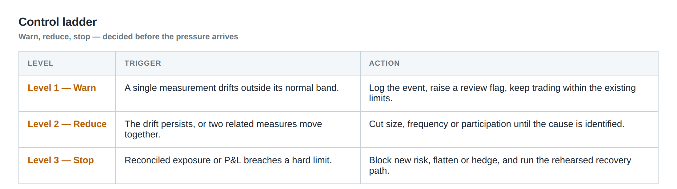
Effectiveness is assessed by three complementary metrics: stale‑order frequency, exposure‑duration loss, and acknowledgement latency tail. Stale‑order frequency counts the number of times an order remained in the venue’s queue after the signal’s TTL had elapsed, regardless of whether it was filled. Exposure‑duration loss quantifies the realised P&L attributable to the interval between TTL expiry and cancel ACK, typically expressed in basis points per trade. A low‑frequency, low‑loss profile indicates that the lifetime guard and synchroniser are operating as intended.

Latency tail measurement requires a high‑frequency timestamping infrastructure that records the full path of each order and its corresponding cancel. By constructing empirical cumulative distribution functions (ECDFs) for order‑to‑ACK and cancel‑request‑to‑ACK intervals, the desk can verify that the 99th percentile remains comfortably below the maximum signal age. If the tail begins to creep upward, the control parameters – such as the guard’s pre‑emptive cancel threshold – must be tightened.

A further diagnostic is the “queue‑value decay curve”. By logging the expected spread capture and adverse‑selection cost at each millisecond of queue residence, the system can plot how quickly the order’s theoretical profit declines. When the curve crosses zero, the order is, by definition, stale. The proportion of orders that cross zero before the TTL is a direct indicator of how well the maximum‑age parameter matches the real market dynamics.

The portfolio view

From a portfolio‑management perspective, each stale order contributes to an invisible risk bucket that can erode the Sharpe ratio over time. Aggregating the exposure‑duration loss across all strategies yields a “latency‑drag” metric, expressed as a percentage of total gross P&L. If latency‑drag exceeds a threshold – for instance, 0.5 % of gross returns – the desk must re‑evaluate its infrastructure, including network paths, co‑location arrangements, and venue‑specific cancel policies.

Moreover, the lifetime discipline imposes a uniform risk horizon across disparate strategies, simplifying capital allocation. By ensuring that every order is bound by a signal‑specific TTL, the desk can model the portfolio’s expected turnover and cash‑flow requirements more accurately. The controls described above also provide a transparent audit trail: each order record contains the signal timestamp, the TTL, the cancel request time, and the venue ACK time. This traceability is essential for post‑trade analysis, regulatory reporting, and for convincing senior management that the latency risk has been quantified and mitigated.

In practice, the portfolio manager should receive a daily summary that lists the number of orders that outlived their TTL, the total loss incurred from those events, and the average cancel‑ACK latency. When the summary shows a consistent downward trend, confidence in the latency‑risk framework grows; when spikes appear, they trigger an immediate review of the underlying network or venue conditions.

Do you currently enforce a maximum age on every signal, and can you quantify the loss that arises when an order survives beyond that age?

About the research behind this lesson

The seminar frames electronic markets as price-time-priority queues. It separates queue value into spread capture versus adverse-selection cost and the option value of retaining a place in line.

Applied to this lesson: An order lifetime therefore cannot be based on elapsed time alone: the system must reassess whether its queue position, expected spread and adverse-selection risk still justify keeping the order alive.

Two live systems, one desk

PULSE-X — power-packed HFT: high-frequency momentum on XAUUSD and EURUSD. System details · Live account

NIC-X — ultra-low drawdown: displaced-print arbitrage for large capital. System details · Live account

Start now: leave your email and request a free trial — we will send the pricing, the connection route and the trial terms. Pricing

Join the market discussion: Telegram @squawklive

Source: High-Frequency Trading and Modern Market Microstructure

Educational content only. Trading leveraged products involves risk.