November 4, 2026

⛶

What this problem really is

In electronic execution the moment an order leaves the strategy and reaches the gateway it becomes a point of exposure that is no longer under the direct control of the model. The exposure is not a single scalar – it is a vector of quantity, notional value, price distance from the mid‑quote and the time the order will remain in the limit‑order book. A naïve threshold that only caps the size of a single order can be bypassed when the same strategy has already accumulated correlated positions elsewhere in the book. The resulting net risk may exceed the portfolio‑wide limits even though each individual order appears compliant.

The difficulty is compounded by the fact that order‑entry pipelines are often decoupled from the risk engine by a few milliseconds. In that window a software bug, a data‑feed latency spike, or a runaway loop can generate a flood of orders that each pass the “maximum quantity” check but together create a dangerous concentration. The problem is therefore not just about a single order, but about the cumulative effect of many orders that share a risk factor.

A second layer of the problem is the quality of the market data that drives the decision. If a signal is produced from a snapshot that is already stale, the price distance check will be misleading, and the order may cross a spread that is no longer available, exposing the strategy to adverse‑selection costs.

How the mechanism works, step by step

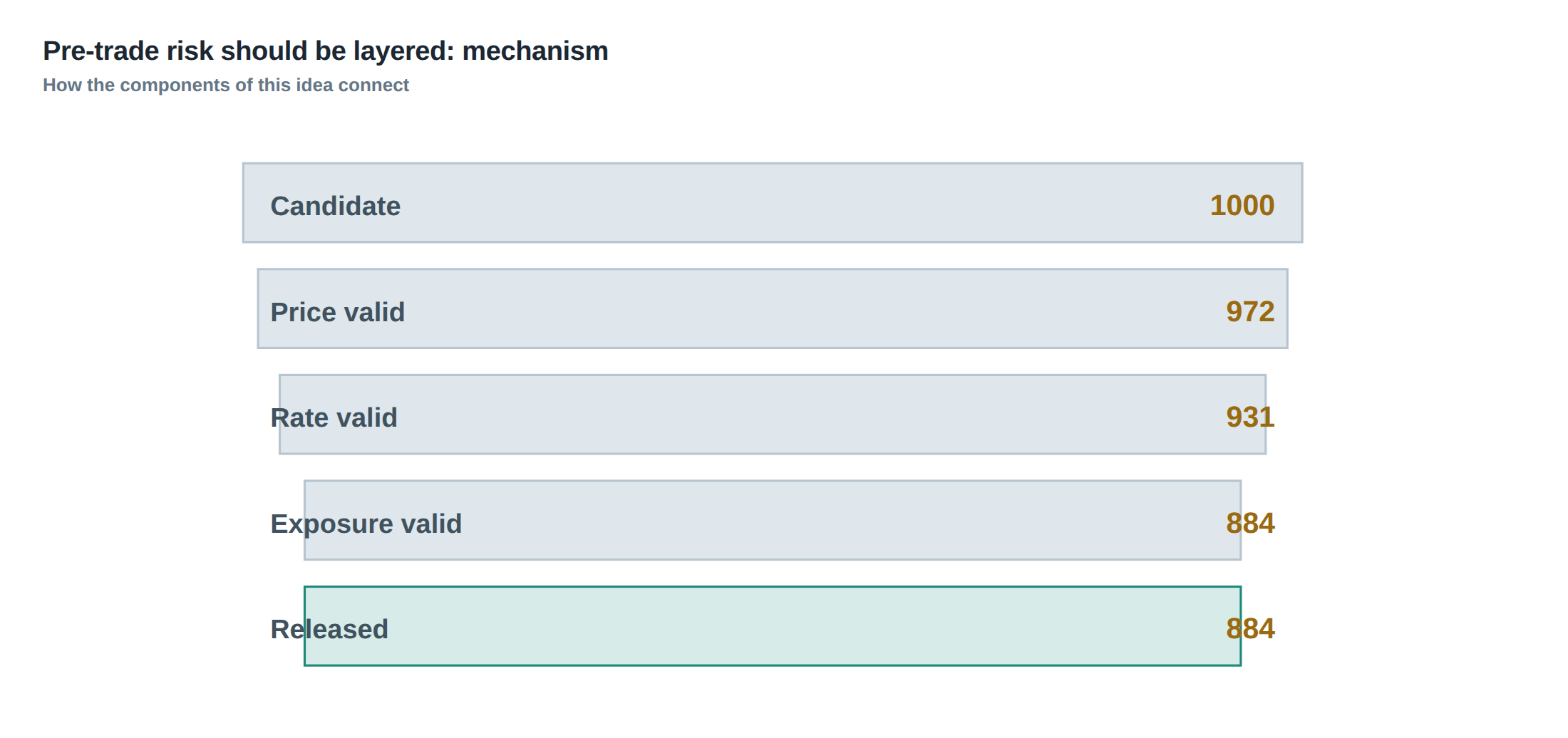
When a signal is generated the first gate is a sanity filter that validates the raw parameters: the intended quantity, the notional value calculated from the last known mid‑price, and the intended price offset from the best bid or ask. The filter also checks the elapsed time since the market data timestamp; if the data is older than a configurable horizon the signal is rejected outright.

If the signal passes the sanity filter it is handed to the risk engine. The engine aggregates the proposed trade with the current exposure across four dimensions: strategy‑level, instrument‑level, account‑level and firm‑wide. For each dimension a pre‑defined ceiling is compared against the sum of existing exposure plus the proposed addition. If any ceiling would be breached the order is rejected before it ever reaches the gateway.

Assuming the order survives the aggregated exposure test, a second risk module examines the order’s expected lifetime in the queue. It estimates the probability of execution based on the current depth, the distance from the best price, and the historical fill‑rate for similar orders. If the expected fill‑rate falls below a threshold, the order is either cancelled immediately or re‑priced to improve its queue position.

Finally the order is passed to the messaging throttler. The throttler limits the frequency of identical messages per second and caps the number of re‑submissions for the same order ID. This prevents a runaway loop from overwhelming the gateway with duplicate requests.

A worked example with real numbers

Consider a statistical arbitrage strategy that trades a basket of three equities: ABC, DEF and GHI. The strategy has a per‑instrument exposure limit of £2 million, a strategy‑level limit of £5 million, and a firm‑wide limit of £20 million. At 09:30:12 the model generates a signal to buy 10 000 shares of ABC at £101.00, sell 8 000 shares of DEF at £50.50 and sell 5 000 shares of GHI at £200.00.

The raw quantities are well under the maximum order size of 50 000 shares, and the notional values are £1.01 million, £404 000 and £1 million respectively – each below the per‑instrument cap. The aggregated exposure after adding the three legs would be £2.414 million for the strategy, still under the £5 million limit, and the total firm exposure would rise to £12 million, well under the £20 million ceiling.

However, the risk engine also tracks correlated exposure across the basket. Earlier in the session the strategy had accumulated a short position of 12 000 shares of ABC at an average price of £102.00, and a long position of 9 000 shares of DEF at £49.80. The net delta of the basket is therefore already biased towards a short exposure on ABC and a long exposure on DEF. Adding the new legs would push the net delta on ABC to a net long of 2 000 shares (10 000 – 12 000) and on DEF to a net short of 1 000 shares (8 000 – 9 000). The risk model flags that the combined delta on the ABC‑DEF pair exceeds the pairwise correlation limit of £1.5 million, even though each leg individually respects its limit. Consequently the order is rejected.

The rejection is logged with a code that indicates “correlated exposure breach” and is streamed to the operations dashboard for immediate visibility.

Where it breaks in live markets

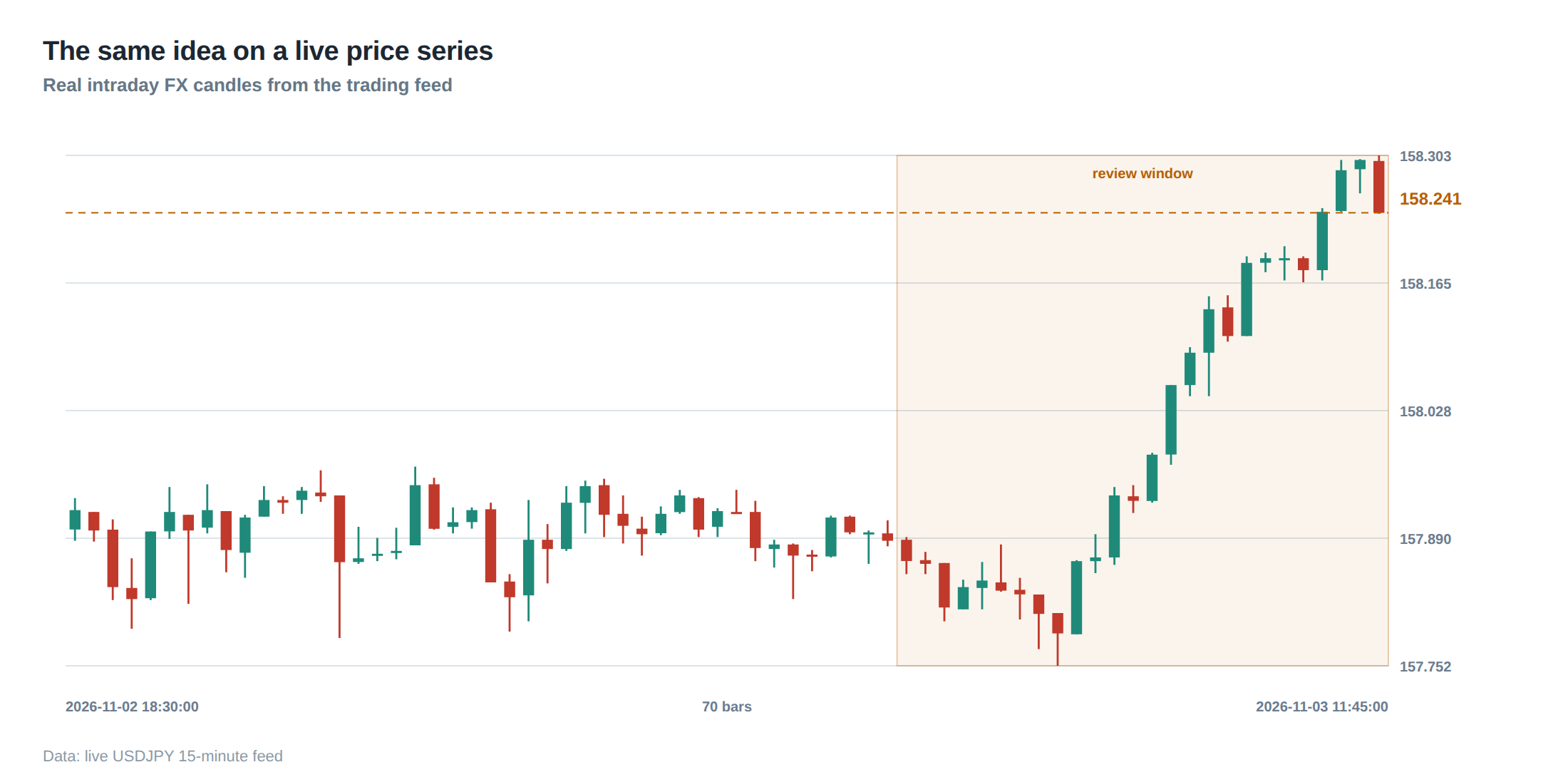
In a live environment the most common failure mode is the decoupling of market‑data timestamps from order‑submission timestamps. A latency spike of 150 ms can cause the strategy to act on a price that has already moved two ticks, turning a modest price‑distance check into a hidden crossing of the spread. The order then sits in the queue with an adverse‑selection cost that far exceeds the original risk budget.

Another break point is the “burst” scenario where a software bug causes the same signal to be emitted repeatedly. The throttler may be configured with a limit of 5 messages per second, but a bug that generates 20 identical messages per second will still see the first five pass the throttler before the excess are dropped. The five that slip through may each be for a different instrument, yet collectively they can saturate the instrument‑level limit in a matter of seconds.

A third source of failure is the mis‑alignment of the exposure aggregation windows. If the risk engine aggregates on a rolling 1‑second window but the order‑gateway processes messages on a 5‑second batch, the exposure snapshot used for the check may be stale, allowing a temporary overshoot that is later corrected only after the orders have already been placed.

The operating path, stage by stage

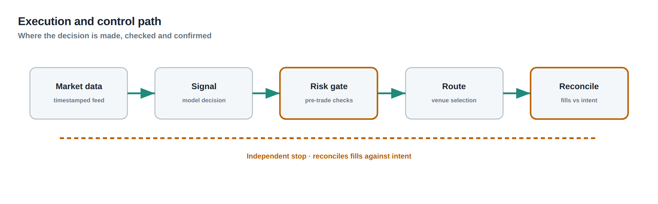
The first stage is the signal generator, which outputs a JSON payload containing the instrument, side, quantity, target price and a timestamp. The second stage is the pre‑trade sanity filter that validates the payload against static limits on quantity, notional value and price distance, and discards any payload older than the data‑age threshold. The third stage is the aggregated exposure engine, which pulls the latest position book, applies the correlation matrix, and calculates the projected exposure for each of the four hierarchy levels. The fourth stage is the queue‑value estimator, which uses the current depth of the limit‑order book to compute the expected fill probability and the adverse‑selection cost. The fifth stage is the messaging throttler, which enforces per‑instrument and per‑strategy rate limits and suppresses duplicate submissions. The final stage is the gateway interface, which translates the approved order into the exchange‑specific protocol and acknowledges success or failure back to the strategy.

Each stage produces a deterministic audit record that is appended to a central log. The log is consumed by a real‑time monitoring service that raises alerts when any rejection code is emitted, and it also feeds a daily risk‑reconciliation batch that checks for any exposure drift.

Controls that act before the damage

The first line of defence is the static sanity filter, which is deliberately simple and fast to execute. It checks that the quantity does not exceed the maximum order size, that the notional value stays within the instrument‑level cap, and that the price offset is no greater than a pre‑set multiple of the current spread. It also validates the data timestamp, rejecting any signal older than the configured staleness window.

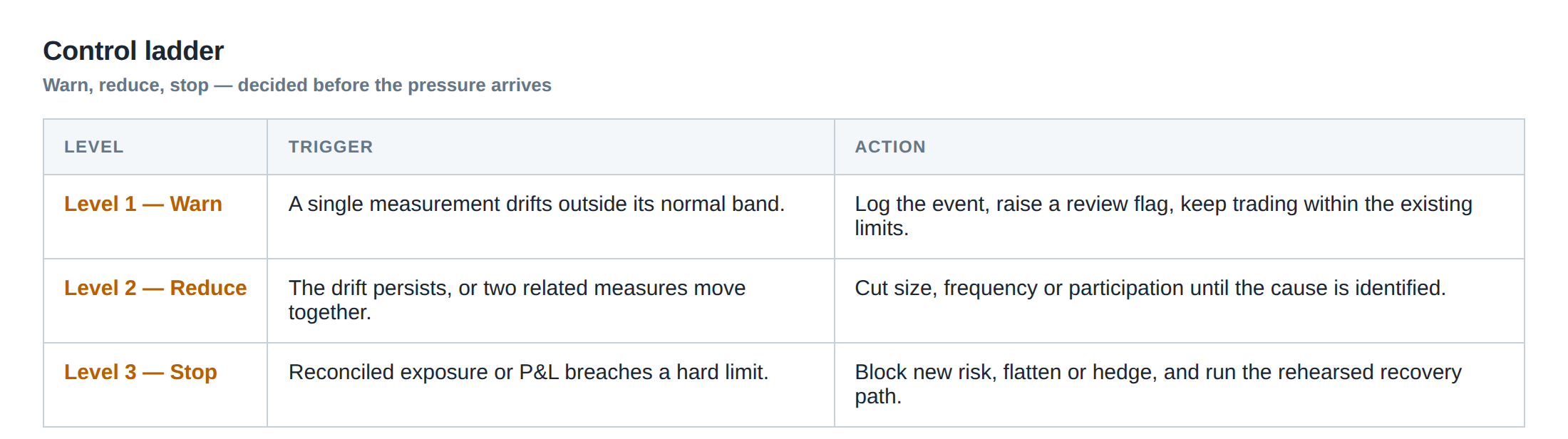
The second defence is the exposure ladder. At the base of the ladder sit the per‑instrument limits; above them sit the strategy‑level limits; next are the account‑level limits; and at the top sits the firm‑wide limit. An order must clear each rung before it can proceed. The ladder is dynamic: if the market moves sharply and the correlation matrix is updated, the limits on the intermediate rungs are automatically tightened for the affected instruments.

The third defence is the queue‑value monitor. It continuously recomputes the expected spread capture and adverse‑selection cost for every live order. If the expected net benefit falls below a configurable threshold, the order is cancelled or re‑priced. This prevents an order from lingering in the book long after the market conditions that justified it have disappeared.

The fourth defence is the message‑rate limiter. It caps the number of order‑submission messages per second per instrument and per strategy, and it tracks repeated attempts to amend the same order. If the same order is amended more than three times within a ten‑second window, the system flags a potential runaway and forces a manual review.

All rejections generated by these controls are broadcast to the operations floor via a low‑latency pub‑sub channel, ensuring that every stakeholder can see the reason for a trade being blocked.

How to measure whether it is working

The primary metric is the “rejection‑to‑submission ratio” measured per hour for each strategy. A stable, low ratio (below 0.5 %) indicates that the pre‑trade checks are aligned with the strategy’s normal behaviour, while a sudden rise suggests either a change in market conditions or a malfunction in the signal generator.

A second metric is the “exposure breach frequency”. This tracks the number of times the aggregated exposure engine would have allowed an order that later caused a portfolio‑level breach. The goal is zero breaches; any non‑zero count triggers an immediate investigation.

Thirdly, the “average queue‑value decay” measures how quickly the expected spread capture for live orders falls after placement. A rapid decay indicates that the queue‑value monitor is correctly cancelling orders that have become unprofitable.

Finally, operational teams monitor the latency of the audit log pipeline. If the time between order rejection and its appearance on the operations dashboard exceeds 200 ms, the visibility loop is compromised, reducing the effectiveness of the controls.

The portfolio view

From the portfolio perspective the layered pre‑trade risk framework acts as a set of overlapping safety nets. The static sanity filter removes the most obvious outliers, the exposure ladder ensures that no single dimension can be overrun, the queue‑value monitor guards against time‑dependent deterioration, and the throttler prevents pathological message storms.

Because each net is evaluated independently, the portfolio can tolerate occasional failures in one net without catastrophic loss, provided the others remain intact. This redundancy is essential in a high‑frequency environment where micro‑second delays can translate into millions of pounds of unintended exposure.

The cumulative effect is a portfolio that evolves within a well‑defined risk envelope, even as individual strategies push the envelope of speed and complexity. By observing the rejection codes, exposure metrics and queue‑value signals in real time, the risk team can intervene before a small coding error or data latency propagates into a systemic event.

Do you have a systematic way of turning each rejection into a learning loop for your strategies?

About the research behind this lesson

The seminar frames electronic markets as price-time-priority queues. It separates queue value into spread capture versus adverse-selection cost and the option value of retaining a place in line.

Applied to this lesson: An order lifetime therefore cannot be based on elapsed time alone: the system must reassess whether its queue position, expected spread and adverse-selection risk still justify keeping the order alive.

Two live systems, one desk

PULSE-X — power-packed HFT: high-frequency momentum on XAUUSD and EURUSD. System details · Live account

NIC-X — ultra-low drawdown: displaced-print arbitrage for large capital. System details · Live account

Start now: leave your email and request a free trial — we will send the pricing, the connection route and the trial terms. Pricing

Join the market discussion: Telegram @squawklive

Source: High-Frequency Trading and Modern Market Microstructure

Educational content only. Trading leveraged products involves risk.