October 14, 2026

What this problem really is

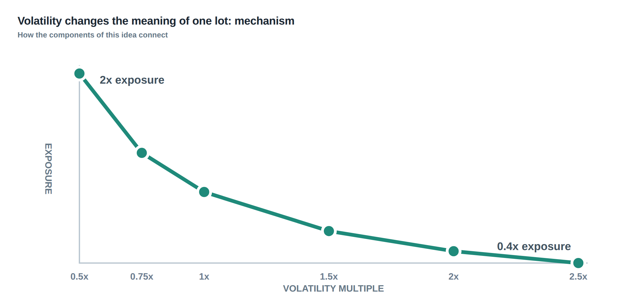
A “lot” in a proprietary desk is usually defined as a fixed number of contracts, shares or notional dollars. The intuition is simple: buying one lot of a futures contract always means the same exposure to price moves. In practice the exposure is a product of the lot size and the instrument’s volatility. When the typical price swing widens, the same lot now carries a larger standard‑deviation of profit and loss, and the risk budget that was calibrated for a quieter regime is instantly breached. The problem is therefore not a question of “how many contracts should I hold?” but “how much volatility does the market currently exhibit and how should that reshape the size of the lot I am willing to trade?”

If the volatility estimate is treated as a static input, the desk’s risk model becomes a brittle slab that cracks whenever the market regime shifts – for example during earnings releases, macro‑policy announcements or the onset of a flash crash. The consequence is an unstable realised risk profile: the same position that historically generated a 0.3 % daily standard deviation may suddenly generate 0.9 % simply because the underlying instrument has entered a high‑variance state. The core thesis, therefore, is that a fixed quantity produces unstable risk when the instrument’s typical movement changes. The solution is to let the lot size be a function of a robust, timely volatility estimate.

How the mechanism works, step by step

The first step is to obtain a forward‑looking volatility estimate that reflects the most recent price dynamics. A common approach is to compute the realised standard deviation of log‑returns over a rolling window – for instance the past 20 minutes for a high‑frequency strategy, or the past 30 days for a medium‑term statistical arbitrage. The window length is a trade‑off: a short look‑back reacts quickly to regime changes but produces noisy estimates, while a long look‑back is smoother but lags behind sudden spikes. The chosen horizon should balance responsiveness against turnover, because each change in the estimate will trigger a re‑scaling of position size.

Once the estimate, σ̂, is in hand, the desk applies an inverse‑volatility rule to compute the target notional: N_target = B/σ̂, where B is the pre‑agreed risk budget expressed in volatility‑adjusted units (for example a 0.5 % daily VaR). The resulting N_target is then rounded to the nearest integer multiple of the contract’s lot size. Floors and caps are imposed to prevent absurdly large or vanishingly small positions – for instance a minimum of one contract and a maximum of 50 contracts for a given instrument. The final order size is the product of the lot multiplier and the rounded N_target.

A worked example with real numbers

Assume the desk trades the E‑mini S&P 500 futures, where one contract represents a notional of US$50 000. The risk budget for the strategy is set at 0.5 % of the portfolio’s equity per trade, which translates to a daily VaR of US$5 000 on a US$1 million capital base. Over the previous 20 minutes the realised volatility of 5‑minute returns is measured at 0.8 % (σ̂ = 0.008). Applying the inverse‑volatility rule gives N_target = 5 000 / (0.008 × 50 000) = 12.5 contracts. After rounding and respecting the floor of one contract, the desk sends an order for 12 contracts, i.e. a total notional of US$600 000.

Now suppose a macro announcement causes the realised volatility to double to 1.6 % (σ̂ = 0.016) while the risk budget remains unchanged. The same calculation yields N_target = 5 000 / (0.016 × 50 000) = 6.25 contracts, which rounds to 6 contracts – a 50 % reduction in exposure. The example illustrates the core thesis: a fixed lot size would have left the desk holding a position whose VaR had jumped from US$5 000 to US$10 000, whereas the volatility‑scaled rule automatically halves the exposure, keeping realised risk within the intended envelope.

Where it breaks in live markets

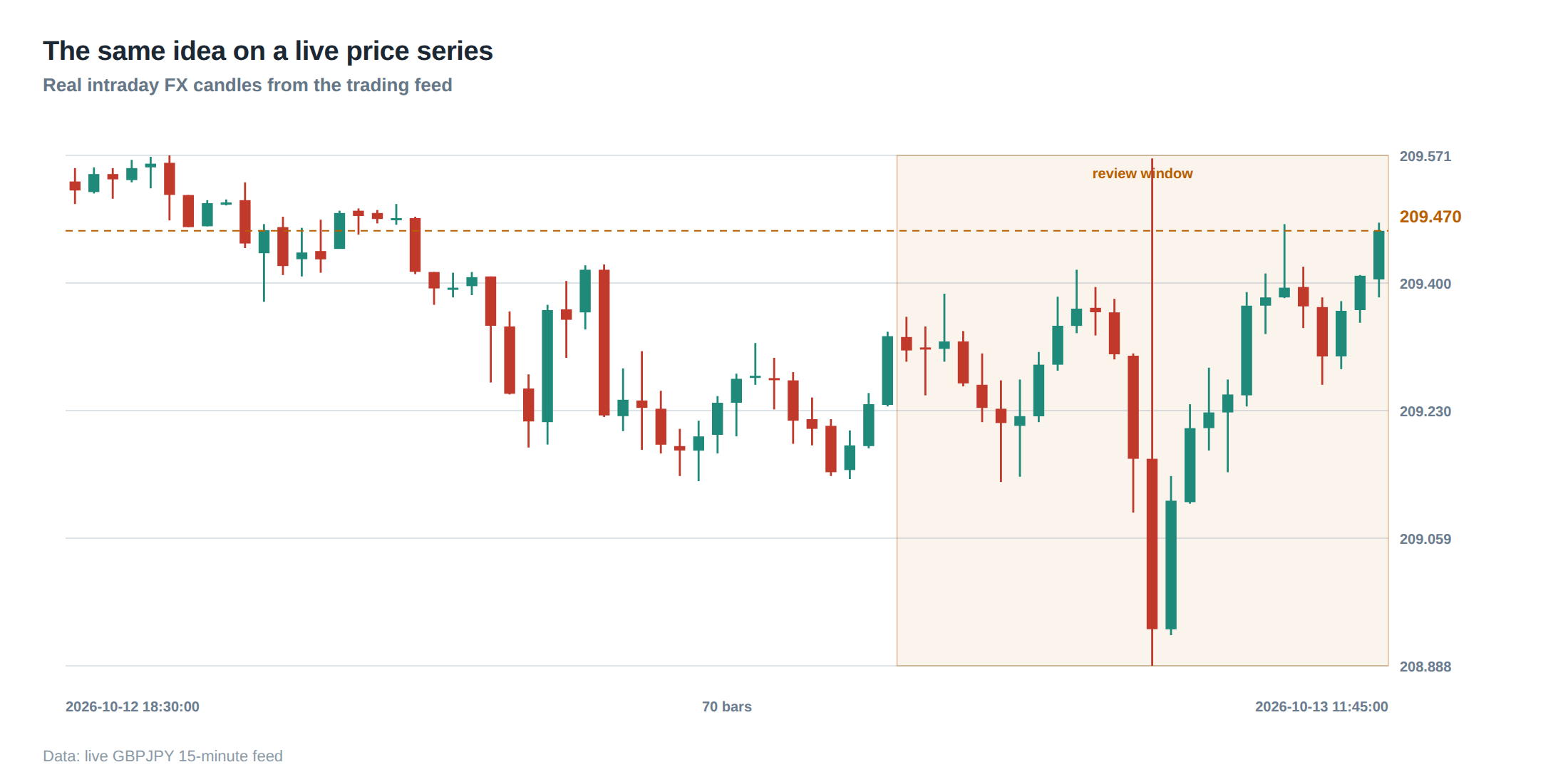
The elegance of the inverse‑volatility rule masks several practical failure modes. First, volatility estimates can become unreliable during market discontinuities such as trading halts, circuit‑breaker trips, or when liquidity evaporates. In those moments the return series may contain outliers that inflate σ̂ dramatically, leading the algorithm to shrink the position to the floor of one contract – potentially missing a profitable move or, worse, leaving the desk under‑hedged. Second, the look‑back window may capture stale price information if the market switches to a new regime faster than the window can adapt, causing the size to lag behind the true risk level. Third, the rule assumes that volatility is the sole driver of risk, ignoring order‑execution pathologies such as tail latencies, stale‑order frequency, or abnormal cancellation‑routing behaviour that can convert a modest position into a tail loss.

The research underpinning modern risk analysis stresses that a single realised outcome cannot fully describe risk; the distribution of returns, including its tails, must be examined. For a fast‑moving strategy, the median latency of order submission is insufficient – the desk must also monitor the frequency of extreme delays, the proportion of orders that become stale, and the loss distribution when the routing infrastructure behaves abnormally. Ignoring these factors creates a blind spot that can turn a well‑scaled position into a catastrophic loss when the market environment deteriorates.

The operating path, stage by stage

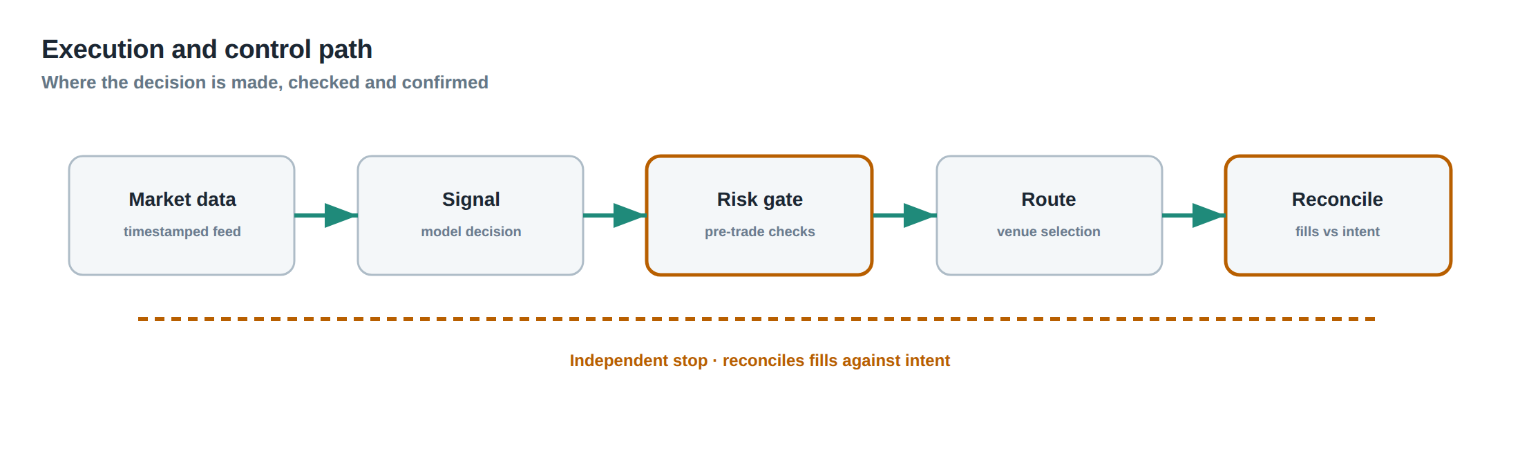
The operational workflow begins with data ingestion: tick‑by‑tick price streams are fed into a rolling‑window calculator that updates σ̂ in real time. The updated volatility is then passed to the position‑sizing engine, which applies the inverse‑volatility formula, enforces the pre‑defined floor and cap, and produces a target contract count. A separate risk‑monitoring module checks the target against additional constraints – for example maximum aggregate exposure across correlated instruments – before the order is handed to the execution gateway. The gateway translates the contract count into a series of limit or market orders, while a latency‑watchdog records the time taken from signal generation to order acknowledgment.

If any of the pre‑trade checks fail – for instance the volatility estimate exceeds a hard upper bound or the latency watchdog flags a tail delay – the engine aborts the order and raises an alert. Otherwise the order proceeds, and post‑trade analytics record the realised P&L, the actual execution price, and the realised volatility over the holding period. These realised figures are fed back into the risk‑budget calculator to adjust B if necessary, completing the feedback loop. The flow ensures that each stage can intervene before an oversized position is allowed to trade, and that the system continuously learns from the outcome of each trade.

Controls that act before the damage

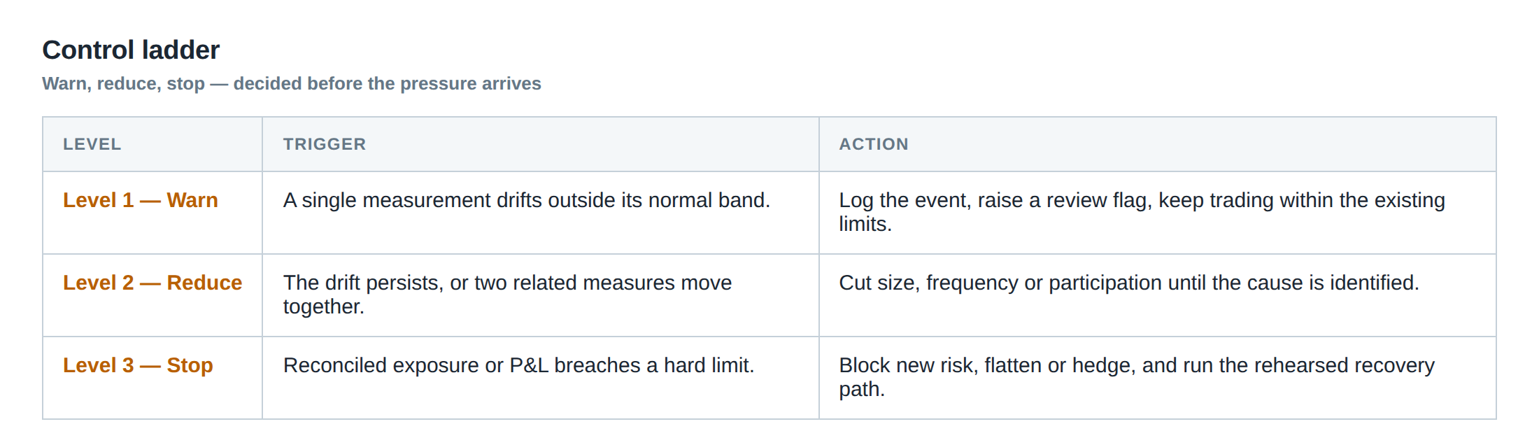
Pre‑trade controls are layered to prevent the volatility‑scaled size from becoming a source of ruin. The first line is the volatility floor and cap, which guarantee that σ̂ cannot be driven to zero (which would produce an infinite position) nor allowed to explode beyond a pre‑set maximum (which would force the size to the minimum lot). The second line is a regime‑filter that monitors market micro‑structure health – for example the proportion of orders that are rejected, the depth of the order book, and the frequency of quote‑stale events. When the filter detects a deteriorating environment, it forces the size down to the minimum contract or temporarily disables new entries.

A third safeguard is the execution‑quality monitor. It records tail latencies – the 99th percentile of time between order submission and acknowledgement – and compares them against a threshold derived from historical performance. If the tail latency breaches the threshold, the system automatically reduces the target size by a predefined factor, often 30 % to 50 %, until latency returns to acceptable levels. Finally, a manual oversight panel receives real‑time dashboards summarising volatility, size, and execution metrics, allowing a trader or risk manager to intervene if the automated logic appears to be misbehaving.

How to measure whether it is working

Effectiveness is assessed by comparing the realised risk of the volatility‑scaled positions against the original risk budget. The primary metric is the realised VaR or expected shortfall (ES) calculated on the daily P&L series of the strategy, expressed as a percentage of equity. If the realised VaR consistently stays below the allocated B, the scaling rule is deemed successful. A secondary check is the turnover ratio: the number of contract adjustments per day divided by the average open contracts. Excessive turnover may indicate that the look‑back window is too short, while very low turnover could suggest that the volatility estimate is lagging.

Execution quality provides another diagnostic. The distribution of slippage – the difference between the intended price and the actual execution price – should be examined for heavy tails. A widening tail after a volatility spike signals that the size reduction may not have been sufficient to offset execution risk. Finally, the system logs the frequency of pre‑trade aborts triggered by the regime‑filter or latency watchdog; a rising trend could be an early warning that market conditions are entering a phase where the current volatility model no longer captures the true risk.

The portfolio view

When each instrument in a multi‑asset portfolio is scaled independently by its own volatility estimate, the aggregate risk profile becomes a function of the correlation structure as well as the individual volatilities. The desk therefore aggregates the scaled notional exposures into a covariance matrix, applying a factor model or a full‑sample estimator to compute the portfolio‑wide VaR. This step reveals whether the volatility‑scaled positions are inadvertently concentrating risk in a particular sector or time‑zone.

If the portfolio VaR exceeds the global risk limit, the desk can apply a secondary scaling factor – a portfolio‑level multiplier – that uniformly shrinks all positions until the limit is respected. This hierarchical approach preserves the relative size decisions made at the instrument level while ensuring that the overall risk remains bounded. Continuous monitoring of realised portfolio volatility, together with the individual instrument metrics described earlier, provides a comprehensive picture of whether the core thesis – that a fixed lot size leads to unstable risk – has been mitigated across the whole desk.

Do you have a systematic method for choosing the volatility look‑back window that balances responsiveness with turnover in your own trading book?

About the research behind this lesson

Andrew Lo's lectures build risk analysis from return distributions and statistical measures, rather than treating one realised result as a complete description of risk.

Applied to this lesson: For a fast strategy, median latency or average fill quality is not enough. The review has to include tail delays, stale-order frequency and the loss distribution when cancellation or routing behaves abnormally.

Explore PULSE: System details

PULSE live account: Verify the live account on FX Blue

Live chat and updates: Telegram @xtrskhft

Source: Risk and Return

Educational content only. Trading leveraged products involves risk.