October 27, 2026

⛶

What this problem really is

Electronic market participants are accustomed to thinking of risk in terms of a single “stop‑loss” or a per‑order notional ceiling. In practice the failure modes of an automated strategy are far more varied. An order may be correctly sized, priced within the quoted spread and submitted at a time when market data appear fresh, yet still generate a loss that far exceeds the intended exposure because the strategy is already carrying correlated positions that have exhausted the portfolio’s risk budget. The core issue is that a single threshold—whether it be maximum quantity, notional value or price distance—cannot anticipate every combination of order‑side error, data latency, or interaction with existing positions.

At a prop‑trading desk the consequence of such an oversight is not merely a modest slippage but a potential breach of capital limits, margin calls, or regulatory breaches. The problem therefore sits at the intersection of order‑entry validation, real‑time risk aggregation, and operational observability. When an order passes the superficial checks but later proves to be dangerous, the damage is already done; the trade has entered the market, the execution engine has allocated capital, and the downstream risk engine may be forced into a reactive mode.

The solution is to view pre‑trade risk as a layered defence, each layer addressing a different dimension of the problem. The first layer validates the order against static limits – quantity, notional, and price distance. The second layer monitors behavioural patterns such as message frequency and repeated submissions. The third layer aggregates exposure across strategy, instrument, account and firm‑wide scopes. The fourth layer rejects any order that is based on market data older than a configurable freshness window. Finally, every rejection must be recorded in a way that operations can audit, replay and improve the rule set. Only by stacking these layers can a desk protect itself from the combinatorial explosion of order‑error scenarios.

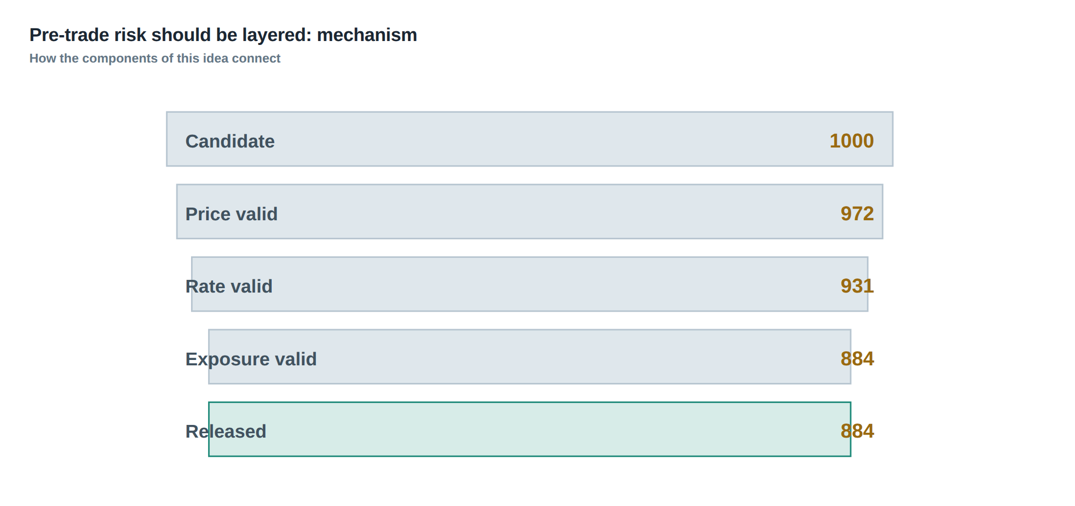
How the mechanism works, step by step

When a signal originates from a strategy, it is first packaged into an order request that contains the intended side, quantity, limit price and a timestamp. The first gate in the pre‑trade chain checks the request against static limits: the quantity must be below the instrument‑specific maximum, the notional value (price × quantity) must not exceed the per‑order ceiling, and the limit price must lie within a pre‑defined distance from the mid‑price – often expressed in ticks or basis points. If any of these checks fails, the request is rejected immediately and a rejection code is emitted.

Assuming the static checks pass, the request proceeds to the behavioural gate. Here the system examines the rate at which the same strategy or the same trading account has submitted orders in the recent window (for example, no more than five orders per second). It also looks for repeated submissions of identical parameters, which can indicate a stuck algorithm or a network retransmission. If the frequency exceeds the threshold, the request is throttled or rejected, and an alert is raised for the operations team.

The third gate aggregates exposure. The risk engine maintains a real‑time view of the net position for each strategy, each instrument, each account and the firm as a whole. It computes the incremental impact of the new order on the existing exposure, taking into account correlation matrices that capture how the new instrument moves with the current portfolio. If the incremental exposure would push any of the pre‑defined limits – for example, a 20 % VaR limit for the strategy or a 10 % concentration limit for the instrument – the order is rejected.

The final gate validates data freshness. Market data timestamps are compared to the order timestamp; if the data are older than the allowed staleness window (often 100 ms for equities, 250 ms for futures), the order is rejected as “stale”. This prevents the system from acting on a price that has already moved, a common source of adverse selection. Each rejection, regardless of the gate that triggered it, is logged with a rich context – strategy identifier, instrument, limit breached, and the exact timestamp – so that operations can trace the decision path and adjust parameters if needed.

A worked example with real numbers

Consider a statistical arbitrage strategy that trades a basket of three equities: X, Y and Z. The firm‑wide notional limit per order is set at $100 000, the maximum quantity per instrument is 500 shares, and the price‑distance limit is five ticks (where one tick equals $0.01). The strategy’s daily VaR budget is $200 000, and the correlation matrix shows that X and Y move together with a coefficient of 0.85, while Z is largely independent.

At 09:30:12.345 the strategy generates a signal to buy 400 shares of X at $250.00, sell 300 shares of Y at $150.00 and buy 200 shares of Z at $45.00. The notional values are $100 000, $45 000 and $9 000 respectively, each below the per‑order ceiling. The price‑distance checks pass because all limit prices are within three ticks of the mid‑price. The behavioural gate sees that this is the third order from the strategy in the last second, well under the five‑orders‑per‑second limit.

The exposure gate, however, reveals a problem. The existing portfolio already holds a long position of 600 shares in X, valued at $150 000, and a short position of 400 shares in Y, valued at $60 000. The new order would increase the net long exposure in X to $250 000 and the net short exposure in Y to $90 000. Using the correlation coefficient of 0.85, the incremental VaR contribution of the X–Y pair is approximately $68 000, pushing the strategy’s total VaR from $140 000 to $208 000, which exceeds the $200 000 budget. Consequently, the exposure gate rejects the entire multi‑leg request, even though each leg individually satisfied the static limits.

If the exposure gate were omitted, the order would have passed the first two layers, entered the market, and the execution of the X leg alone would have consumed the remaining risk budget, leaving the strategy vulnerable to a rapid reversal in X’s price later in the session. The layered approach therefore prevents a situation where an apparently innocuous order becomes dangerous due to hidden correlations.

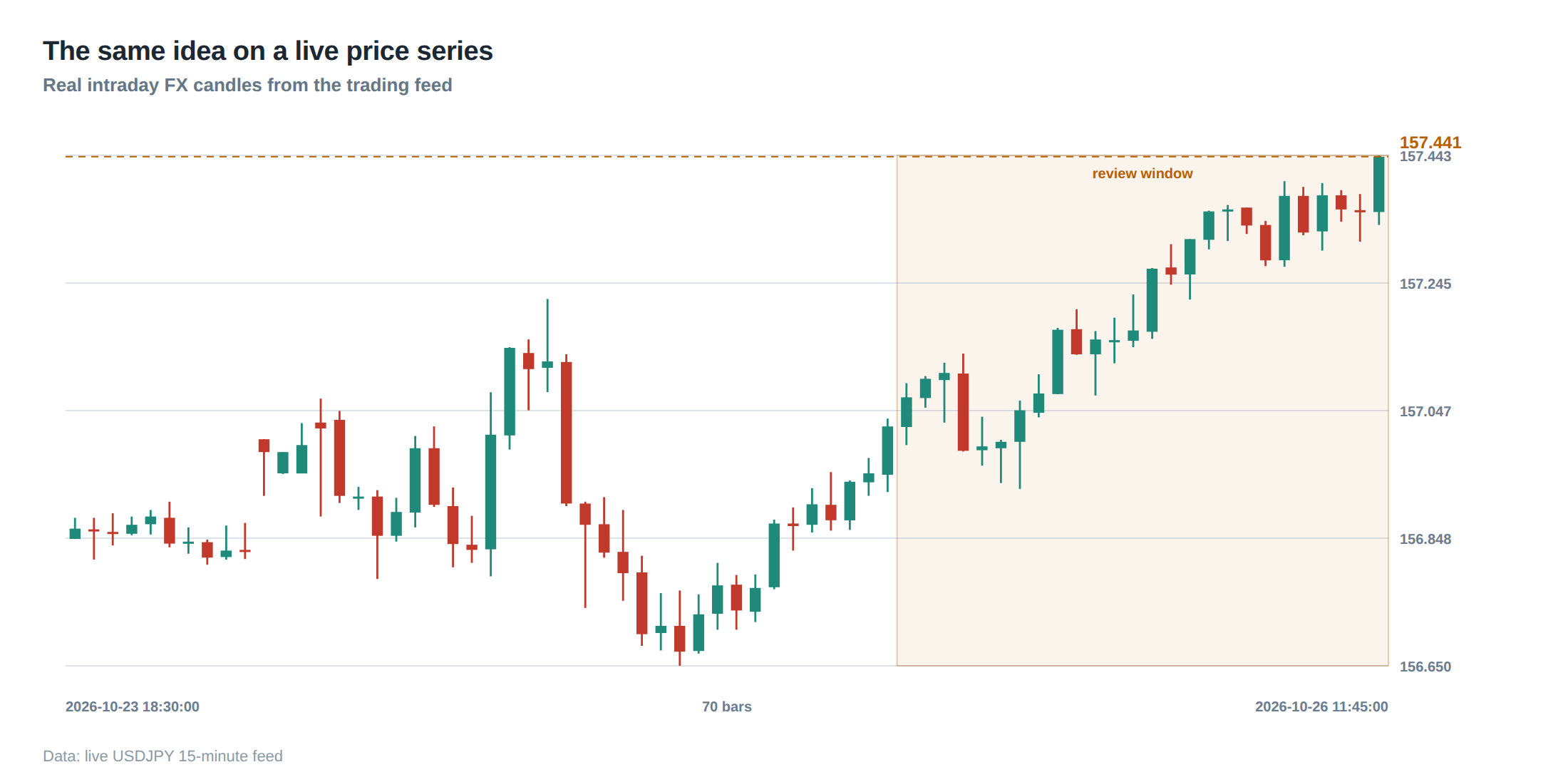
Where it breaks in live markets

Even a well‑designed layered system can be undermined by real‑world frictions. Latency spikes in the market data feed may cause timestamps to drift, making the freshness gate either too permissive or too aggressive. In high‑frequency environments a sudden surge in order flow can temporarily breach the message‑frequency limits, leading to a cascade of rejections that stall the strategy and cause missed opportunities.

Another failure mode is the mismatch between the risk model’s correlation estimates and the actual market dynamics. Correlations can shift abruptly during news events; a model that assumes a stable 0.85 coefficient between X and Y may underestimate the joint risk when both stocks react to a sector‑wide shock. If the exposure gate relies on stale correlation inputs, it may let a dangerous order through.

Operationally, the observability requirement can be neglected. If rejection logs are written to a low‑throughput database, the operations team may not notice a pattern of rejections until after the damage has accumulated. Moreover, if the rejection codes are ambiguous, troubleshooting becomes a manual, time‑consuming process that can delay corrective action.

Finally, the layered approach assumes that each gate is independent, but in practice they interact. For example, throttling order submissions can inadvertently reduce the signal‑to‑noise ratio of the strategy, causing it to generate larger, less frequent orders that stress the exposure gate in a different way. Understanding these interactions is essential for maintaining robustness.

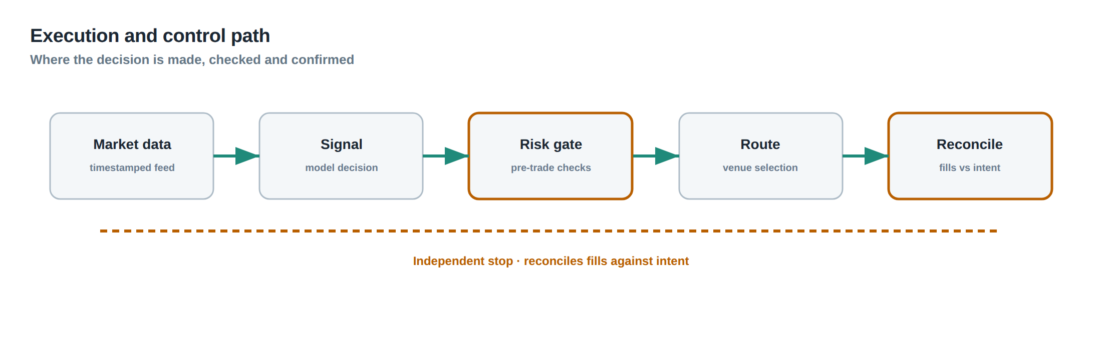
The operating path, stage by stage

The first stage is signal generation, where the algorithm outputs a set of intended trades together with a confidence score and a timestamp. The second stage is order construction, translating the signal into a FIX message that includes quantity, price and a unique identifier. The third stage is static validation, where the system checks the quantity, notional and price‑distance against the instrument‑specific limits.

If the order passes, it proceeds to the behavioural validation stage, which monitors the rate of order creation per strategy and per account, and flags any repeated submissions that exceed the configured thresholds. Successful orders then move to the exposure aggregation stage, where the risk engine updates the net position, computes the incremental VaR, and evaluates concentration limits across all relevant dimensions.

The penultimate stage is data‑freshness validation, which compares the market data timestamp embedded in the order with the latest market snapshot. If the data are older than the allowed latency, the order is rejected. The final stage is the dispatch stage, where the order is sent to the execution venue, and a confirmation is logged. Throughout the path, each rejection is recorded with a structured payload that includes the gate name, the breached parameter and the exact market snapshot used for the decision.

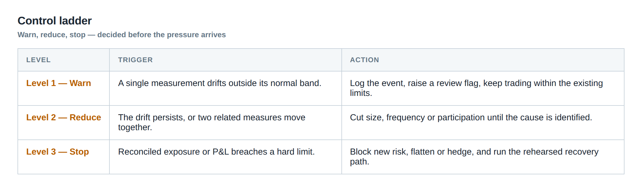
Controls that act before the damage

The first line of defence is the static limit control. By fixing a hard ceiling on quantity, notional and price distance, the system eliminates the most obvious outliers – accidental large orders caused by a coding error or a mis‑configured parameter. The second control is the behavioural throttling, which caps the number of messages a strategy may emit in a short window, thereby protecting the downstream risk engine from being overwhelmed and limiting the opportunity for a runaway algorithm to flood the market.

The third control is the exposure aggregation, which operates on a real‑time ledger of positions. It uses a matrix of pairwise correlations to translate a new order into an incremental risk metric, such as VaR or expected shortfall, and compares this against the pre‑approved budget for the strategy, instrument and firm. Because the calculation is incremental, it can be performed in microseconds, ensuring that the order never leaves the desk if it would breach a limit.

The fourth control is the data‑freshness gate. It discards any order whose market data timestamp is older than a configurable threshold, thereby avoiding the classic “stale quote” problem that leads to adverse selection. The final control is the observability layer: each rejection is emitted as an event to a monitoring pipeline, enriched with context, and stored in an immutable audit log. This enables the operations team to detect systematic issues, such as a recurring breach of a particular limit, and to adjust the parameters before a larger incident occurs.

How to measure whether it is working

Effectiveness can be assessed by tracking the ratio of rejected orders to total generated orders over a rolling window. A stable, low‑to‑moderate rejection rate (for example, 1‑3 % of all orders) indicates that the controls are active without being overly restrictive. More informative is the distribution of rejection reasons; a shift from “static limit” rejections to “exposure” rejections suggests that the portfolio is approaching its risk budget, prompting a review of allocation.

Another metric is the time‑to‑reject. The latency from order creation to final decision should remain well within the market’s microsecond‑level dynamics; any increase signals a bottleneck in the risk engine or in the data‑freshness check. Additionally, the number of “stale‑data” rejections can be correlated with market‑feed latency statistics to verify that the freshness window is appropriately set.

Operationally, the audit log should be queried daily for patterns such as repeated rejections from the same strategy or instrument. The presence of such patterns may indicate a mis‑calibrated parameter or a deeper algorithmic issue that requires developer attention. Finally, a post‑trade analysis should compare the realised P&L of trades that passed all layers against the expected P&L from the model; a systematic deviation could imply that the pre‑trade controls are allowing marginally profitable but risk‑heavy trades to slip through.

The portfolio view

From a portfolio perspective, pre‑trade layering is not an isolated safety net but an integral component of capital allocation. The exposure gate directly enforces the risk budget that the portfolio manager has set for each strategy, ensuring that the aggregate VaR remains within the firm‑wide limit. When a trade is rejected at the exposure stage, the manager receives immediate feedback that the strategy is operating near its capacity, prompting either a reduction in signal generation or a re‑balancing of existing positions.

Because the controls are hierarchical, they also provide a natural hierarchy of alerts. A static‑limit breach typically warrants a quick code review, while an exposure breach may trigger a strategic discussion about market conditions or model assumptions. The data‑freshness rejections feed into the market‑data quality team, who can then investigate latency spikes that may affect multiple desks.

In this way, the layered pre‑trade system aligns the micro‑level order decisions with the macro‑level portfolio objectives, creating a feedback loop that keeps the desk within its risk appetite while preserving the ability to act on genuine opportunities.

Do you think your current pre‑trade validation framework adequately captures the hidden interactions between static limits, behavioural patterns and portfolio‑wide exposure, or could a deeper layering approach reveal blind spots in your risk management?

About the research behind this lesson

The seminar frames electronic markets as price-time-priority queues. It separates queue value into spread capture versus adverse-selection cost and the option value of retaining a place in line.

Applied to this lesson: An order lifetime therefore cannot be based on elapsed time alone: the system must reassess whether its queue position, expected spread and adverse-selection risk still justify keeping the order alive.

Two live systems, one desk

PULSE-X — power-packed HFT: high-frequency momentum on XAUUSD and EURUSD. System details · Live account

NIC-X — ultra-low drawdown: displaced-print arbitrage for large capital. System details · Live account

Start now: leave your email and request a free trial — we will send the pricing, the connection route and the trial terms. Pricing

Live chat and updates: Telegram @xtrskhft

Source: High-Frequency Trading and Modern Market Microstructure

Educational content only. Trading leveraged products involves risk.