October 18, 2026

⛶

What this problem really is

In modern electronic markets the dominant matching rule is price‑time priority. An order that arrives first at a given price level enjoys a queue position that can be monetised through the spread that is captured when the order is filled. The intuition that “faster is always better” rests on the assumption that a reduction in latency translates directly into a better execution price or a higher probability of completion. In practice the relationship is far more fragile. A trader who merely accelerates the order‑submission path without monitoring how often the order is rejected, how much spread is actually realised, or whether the market moves against the trade after the fill may be chasing an illusion. The true edge lies not in raw response time but in the marginal improvement of the economic outcomes that matter: execution price, fill probability, and post‑trade risk.

The problem therefore is a measurement problem as much as a technology problem. Latency can be measured with nanosecond‑precision timestamps, but fill‑rate, realised spread, and the distribution of adverse price moves are stochastic quantities that must be estimated in parallel. When an order is sent to a venue that is already saturated with toxic flow, the latency advantage may be nullified because the order is rejected or because it only reaches the book when the price is already moving unfavourably. A disciplined desk therefore needs a framework that treats latency as a lever that must be calibrated against the marginal gain in executable price and the marginal increase in execution risk.

How the mechanism works, step by step

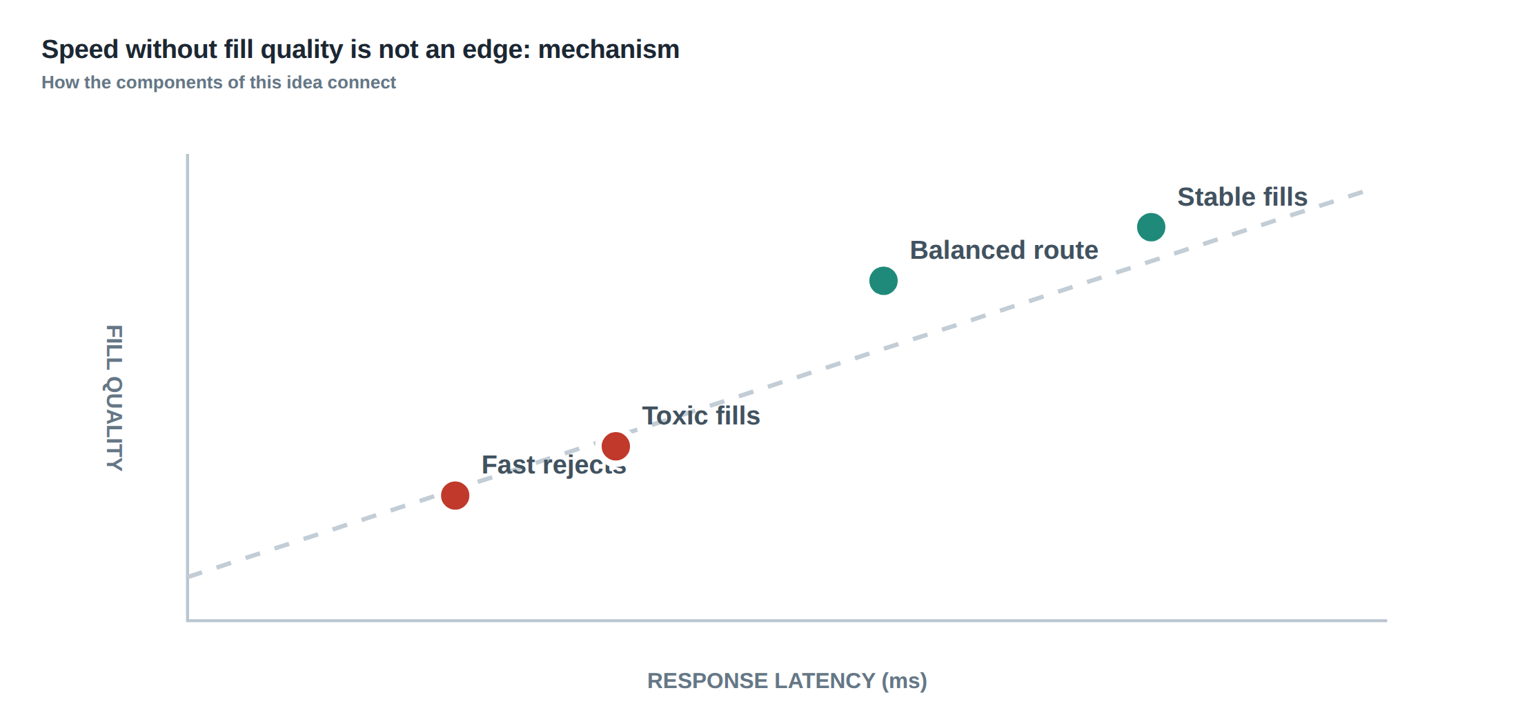
The electronic market can be abstracted as a set of parallel queues, one for each price level on each venue. When a market participant decides to place a limit order, the decision engine first evaluates the expected spread capture at the target price, the probability that the order will survive in the queue, and the adverse‑selection cost that accrues while the order waits. The order is then transmitted through a chain of network hops, each adding a deterministic or stochastic delay. Upon arrival at the gateway, the order is either accepted into the queue, rejected outright (for example because the price is no longer quoted or because the venue’s risk controls fire), or placed into a “soft‑reject” state where it is queued for later routing.

If the order is accepted, it occupies a position in the queue. The value of that position decays over time as other participants submit orders ahead of it, and as the mid‑price drifts. The trader’s system must therefore decide, at each millisecond, whether the remaining expected spread capture still outweighs the risk of being displaced or of the market moving against the position. When the decision engine determines that the expected marginal benefit has fallen below a pre‑defined threshold, it issues a cancellation. The cancellation itself incurs latency, and the speed of that cancellation can be as important as the speed of the original submission.

Crucially, the decision to keep an order alive cannot be based solely on elapsed time. It must incorporate a real‑time reassessment of three variables: (i) the updated queue position, (ii) the realised spread that would be earned if the order were filled now, and (iii) the adverse‑selection cost implied by the recent order‑flow imbalance. When any of these variables deteriorate beyond the edge budget, the order should be withdrawn, regardless of how much time remains in the original “lifetime” window.

A worked example with real numbers

Consider a high‑frequency market‑making strategy that posts a 1‑tick‑wide bid at 10,000 µUSD on a futures contract. The baseline latency from decision to gateway is 12 ms. Historical data show that at this latency the order fills 85 % of the time, with an average realised spread of 0.45 ticks, and a rejection rate of 2 %. The post‑fill price drift, measured over the next 10 ms, is a modest 0.05 ticks adverse on average.

The desk invests in a new network route and upgrades its order‑management software, reducing the round‑trip latency to 7 ms. After the upgrade, the fill rate drops to 80 % and the rejection rate doubles to 4 %. The realised spread collapses to 0.20 ticks because the order now reaches the book only when the order flow is heavily skewed toward the opposite side – a classic “toxic flow” scenario. Moreover, the adverse price movement after a fill widens to 0.12 ticks, reflecting that the order is being executed just as the market is turning.

If the desk simply looked at the 5 ms latency reduction, it might conclude that the change is an improvement. However, when the economic metrics are layered together, the picture reverses. The expected profit per order before the upgrade is

\(0.85 \times 0.45 – 0.15 \times 0.05 = 0.3725\) ticks,

whereas after the upgrade it becomes

\(0.80 \times 0.20 – 0.20 \times 0.12 = 0.112\) ticks.

The net edge has been cut by more than two‑thirds, even though the raw latency figure improved. The example illustrates that cutting five milliseconds is not progress if rejected orders double or the strategy reaches the book only when toxic flow is present. It also highlights why fill‑rate, realised spread, and adverse‑selection cost must be measured alongside response time.

Where it breaks in live markets

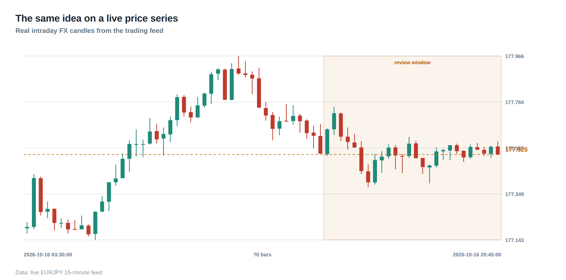
In a live market the theoretical queue model is constantly perturbed by hidden liquidity, iceberg orders, and latency‑arbitrageurs. When a venue experiences a sudden surge in order‑flow volatility – for instance during a macro news release – the queue depth can evaporate within a few milliseconds. An order that would have been filled at the quoted spread under normal conditions may instead be rejected because the venue’s risk engine flags the incoming flow as “excessive”. The same latency advantage that allowed the order to arrive earlier now places it in a regime where the probability of execution is near zero.

Another failure mode is the “price‑drift trap”. If the decision engine bases its placement on a stale mid‑price, a latency reduction may simply bring the order into the market a few milliseconds later, when the price has already moved against the intended side. The order then either sits in the queue for an extended period, accruing adverse‑selection cost, or is cancelled after the market has moved past the original price level, resulting in a missed opportunity.

Venue‑specific quirks also matter. Some exchanges apply a “price‑time‑priority with price‑level protection” rule that penalises orders that arrive after a certain micro‑second threshold, effectively turning a fast order into a slow one if the venue’s internal clock is ahead. In such environments the raw latency figure is misleading unless it is normalised to the venue’s timestamp. The breakdowns above demonstrate that latency must be contextualised against market micro‑structure, not treated as an absolute metric.

The operating path, stage by stage

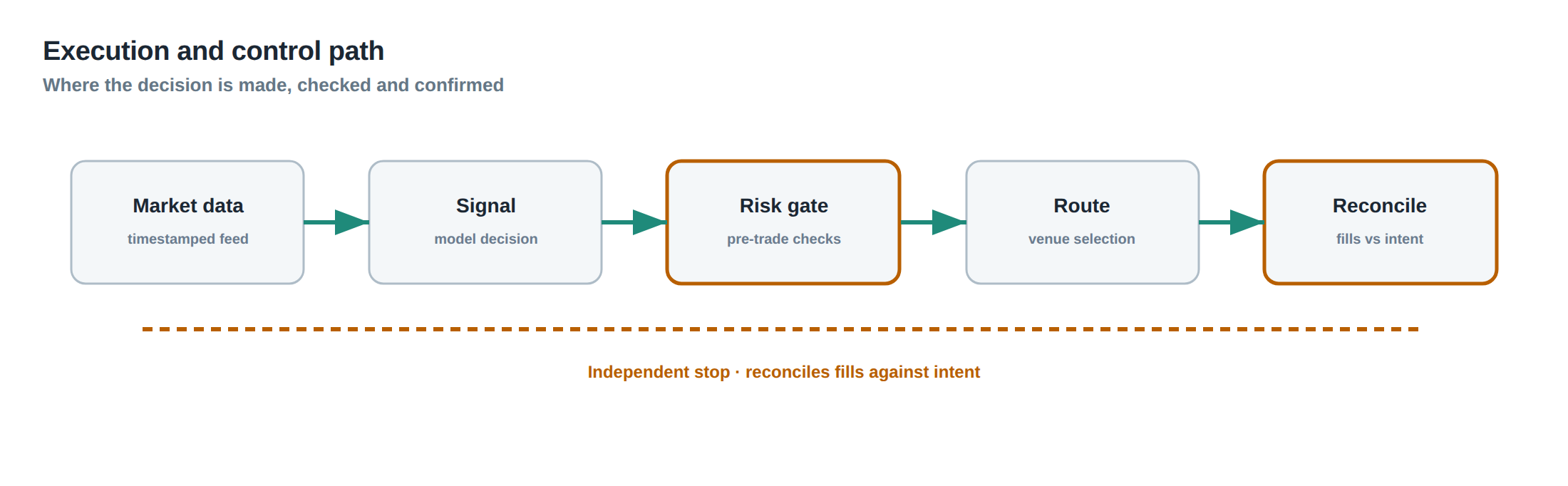
The order journey can be divided into five logical stages. First, the signal generation stage, where the strategy decides whether to trade and at which price. Second, the order‑construction stage, where the order packet is assembled, including any venue‑specific fields such as client order ID or risk‑limit tags. Third, the transmission stage, where the packet traverses the internal network, the data‑center switch fabric, and the external ISP link. Fourth, the gateway‑processing stage, where the exchange’s matching engine validates the order, checks risk limits, and either admits it to the queue or rejects it. Fifth, the post‑execution stage, where the trade is reported, the position is updated, and any post‑trade risk checks are performed.

At each stage, latency is only one dimension of performance. In the signal stage, the quality of the decision (expected spread versus adverse‑selection risk) is paramount. In the construction stage, the completeness of the order fields determines whether the gateway will reject it outright. During transmission, packet loss or jitter can cause retransmissions that inflate effective latency. At the gateway, the order‑book state may have changed between the moment the packet left the desk and the moment it is processed, leading to fast rejections that are indistinguishable from genuine executions without a proper classification. Finally, in the post‑execution stage, the realised spread and subsequent price movement must be recorded to close the loop on the edge calculation.

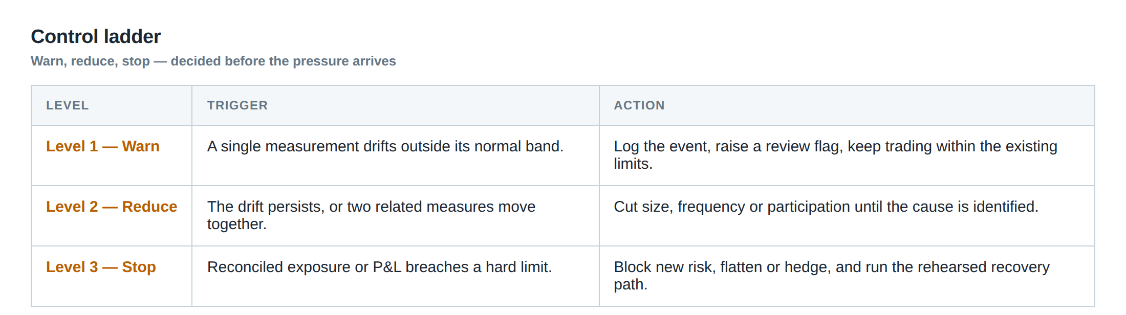
Controls that act before the damage

A robust control architecture places guardrails at each of the five stages described above. Before a signal is emitted, the system applies a “pre‑trade filter” that checks the current order‑flow imbalance, the recent volatility regime, and the venue‑specific queue depth estimate. If the filter flags an elevated adverse‑selection risk, the signal is suppressed. During order construction, a schema validator ensures that all mandatory fields are present and that the order size respects the venue’s per‑order limits, preventing fast rejections that would otherwise waste latency.

In the transmission stage, a “latency‑budget monitor” continuously measures the round‑trip time for heartbeat packets and compares it to a dynamic threshold derived from recent market conditions. When the observed latency spikes, the system can automatically switch to a backup route or throttle order flow to avoid flooding a congested link. At the gateway, a “soft‑reject handler” parses the rejection code in real time; if the code indicates a price‑staleness reject, the handler can instantly adjust the price and resubmit, whereas a risk‑limit reject triggers a back‑off and a risk‑team alert.

Post‑execution, a “realised‑spread calculator” records the execution price, the prevailing best‑bid/ask, and the subsequent mid‑price path for a configurable horizon (e.g., 10 ms, 50 ms). If the realised spread falls below a pre‑set fraction of the expected spread, the system flags the venue or time‑slice for review. Together, these controls act before the damage propagates to the portfolio, ensuring that latency improvements are only realised when they translate into genuine economic benefit.

How to measure whether it is working

Measurement must be multi‑dimensional. First, record the raw latency for every order, from decision timestamp to gateway acknowledgement, using a synchronized clock source such as PTP (Precision Time Protocol). Second, compute the fill‑rate as the ratio of successful executions to total order attempts, separating true fills from fast rejections by inspecting the execution report code. Third, calculate the realised spread for each fill as the difference between the execution price and the contemporaneous mid‑price, expressed in ticks or basis points. Fourth, evaluate the adverse price movement by measuring the mid‑price change over a short horizon after each fill (e.g., 10 ms, 20 ms) and aggregating the results into a distribution.

These metrics should be sliced by venue, trading session (pre‑open, continuous, close), and volatility regime (low, medium, high). A statistical comparison – for example, a two‑sample t‑test of realised spread before and after a latency upgrade – will reveal whether the latency gain has materially improved execution quality. Additionally, a “rejection‑rate per millisecond” curve can highlight whether faster transmission is merely pushing the order into a region of the order book where the venue’s risk engine rejects more aggressively. By monitoring the joint evolution of latency, fill‑rate, realised spread, and post‑fill drift, the desk can confirm that the latency investment is delivering an edge rather than eroding it.

The portfolio view

From a portfolio perspective, the marginal benefit of a latency improvement must be weighed against its marginal cost across all strategies that share the same infrastructure. A strategy that trades a high‑frequency spread‑capture signal may see its edge shrink, while a latency‑sensitive arbitrage strategy might gain a few basis points. The net effect on the portfolio’s Sharpe ratio is the appropriate yardstick. To obtain that view, aggregate the per‑trade profit‑and‑loss contributions after adjusting for transaction costs, then decompose the variance into components attributable to latency‑related execution error versus market risk.

If the latency upgrade leads to a higher variance because of increased adverse‑selection losses on one leg of the portfolio, the overall risk‑adjusted return may fall even though a subset of trades appears faster. Conversely, if the upgrade enables a tighter execution window for a cross‑exchange statistical arbitrage, the reduction in slippage may outweigh the modest rise in rejection‑related costs. The portfolio‑level analysis should be refreshed after any significant change to the network stack, and the results should be benchmarked against a baseline that includes the pre‑upgrade multi‑metric performance. Only when the aggregate risk‑adjusted return improves can the latency investment be justified as an edge.

In practice, this means maintaining a live dashboard that displays, for each strategy, the key metrics outlined above, together with the contribution to overall portfolio volatility and drawdown. Alerts should fire when the realised spread falls below a defined fraction of the expected spread for more than a configurable number of consecutive trades, prompting a review of the latency path.

The portfolio view

In the final analysis, speed without fill quality is a hollow proposition. Latency is a means to an end, not an end in itself. By rigorously measuring fill‑rate, realised spread, rejection patterns, and post‑fill price dynamics, and by embedding these measurements into a disciplined control framework, a prop‑trading desk can ensure that every microsecond saved translates into a measurable improvement in execution economics. The edge resides where the marginal gain in executable price outweighs the marginal increase in execution risk.

Do you have a systematic process for confirming that every latency gain you achieve is reflected in a tangible improvement to realised spread and risk‑adjusted returns?

About the research behind this lesson

The seminar frames electronic markets as price-time-priority queues. It separates queue value into spread capture versus adverse-selection cost and the option value of retaining a place in line.

Applied to this lesson: An order lifetime therefore cannot be based on elapsed time alone: the system must reassess whether its queue position, expected spread and adverse-selection risk still justify keeping the order alive.

Explore PULSE: System details

PULSE live account: Verify the live account on FX Blue

Live chat and updates: Telegram @xtrskhft

Source: High-Frequency Trading and Modern Market Microstructure

Educational content only. Trading leveraged products involves risk.