October 29, 2026

What this problem really is

Statistical‑arbitrage strategies are built on the assumption that two or more securities have a historically stable co‑movement. When the observed spread widens beyond a statistical threshold the trader expects a mean‑reversion profit. The danger is that the historical co‑movement is a model artefact rather than a durable economic relationship. Once capital is allocated, the market can reprice the underlying drivers, the spread can drift indefinitely, or the data feeding the model can become corrupted. In those circumstances the “wide” z‑score that triggered the trade is no longer a signal of convergence but a warning of structural change or data pathology. The resulting loss is not a typical market‑risk event; it is a model‑risk event because the statistical premise itself has failed.

The problem is amplified on a prop‑trading desk where leverage, short‑selling and high turnover are routine. Borrowing costs, funding charges and execution slippage are baked into the P&L from day one, yet they are often treated as secondary to the spread‑capture idea. When the spread does not converge, these costs become a permanent drain that erodes capital even while the position sits idle. The trade‑off between potential convergence profit and the ongoing cost of holding a mis‑specified model is at the heart of the risk.

How the mechanism works, step by step

First, the universe of candidate pairs is filtered by a cointegration test that checks for a stationary linear combination of the log‑prices. The test is run over a rolling window, typically 250 trading days, and the resulting residuals are examined for a half‑life – the time it takes a shock to decay by half. A half‑life of 10‑30 days is usually taken as a sign that the spread reverts quickly enough to be tradable.

Second, the residual series is decomposed into a common‑factor component and an idiosyncratic spread. The common factor is estimated by a principal‑component analysis across the whole basket; the residual after removing this factor is the “pure” spread that the strategy will trade. This step removes market‑wide moves that would otherwise masquerade as convergence opportunities.

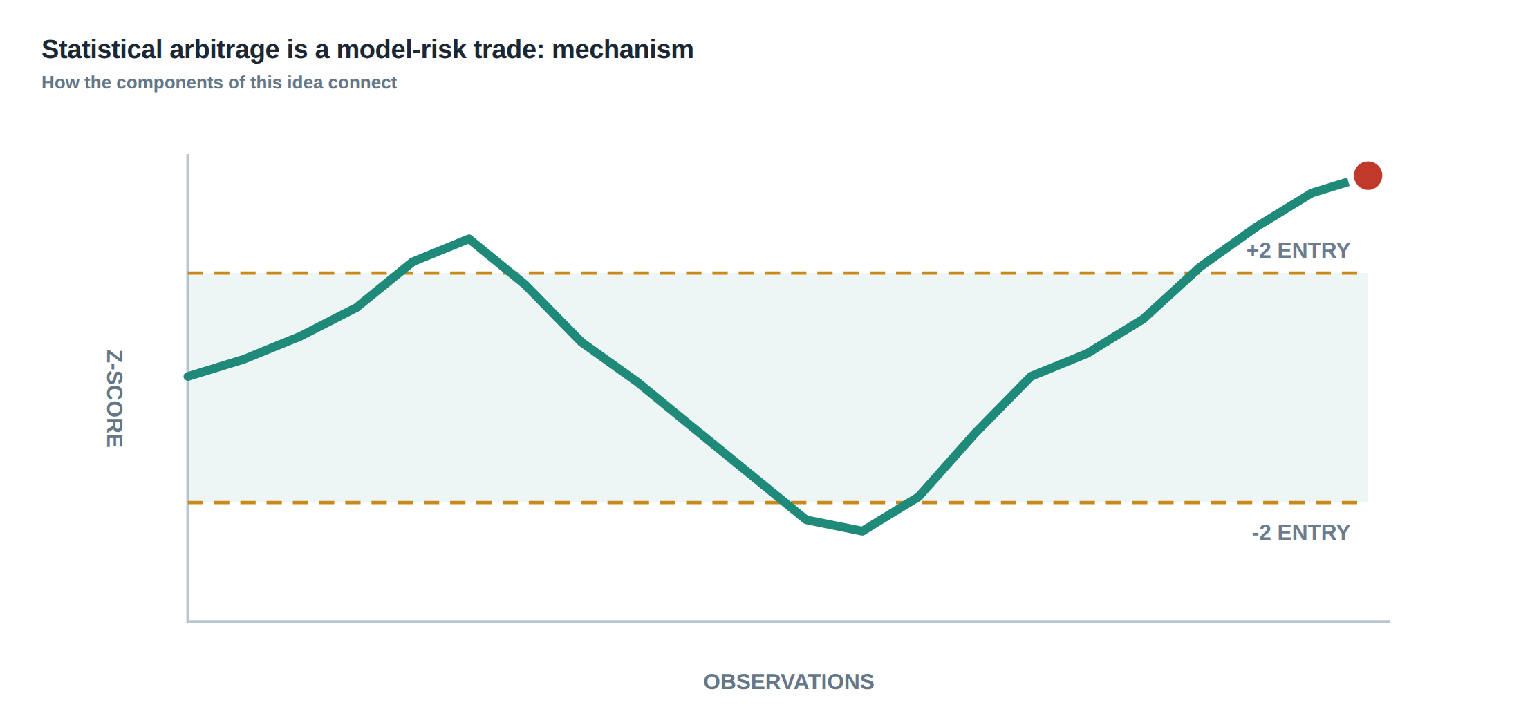
Third, the trader computes a z‑score for the current spread: (current residual – mean) / standard deviation. When the absolute z‑score exceeds a pre‑set threshold (often 2.0), the algorithm generates a signal. The signal is then passed through a cost model that adds borrow rates (e.g. 0.5 % p.a. for the short leg), funding spreads (e.g. 0.2 % p.a. for cash held), turnover cost (estimated 0.10 % per round‑trip) and an execution penalty derived from recent market depth. Only if the expected net profit after these costs exceeds a risk‑adjusted target does the system allocate capital.

Finally, the position is entered with a size that reflects both the signal strength and the uncertainty surrounding it. A wide z‑score of 3.0 could mean a strong reversion signal, but it could also indicate that the underlying relationship has broken down. The model therefore scales the notional down proportionally, for example to 30 % of the maximum allowed exposure, and sets both a price stop (e.g. 1.5 × the historical standard deviation) and a time stop (e.g. 20 trading days) to cap loss if convergence does not materialise.

A worked example with real numbers

Consider a pair of US‑listed technology stocks, AlphaTech (AT) and BetaSystems (BS). Over the past 250 days the log‑price spread \(S_t = \log(P_{AT,t}) – 1.12\log(P_{BS,t})\) has a mean of 0.004 and a standard deviation of 0.018. The Augmented Dickey‑Fuller test on \(S_t\) returns a p‑value of 0.02, indicating stationarity at the 5 % level. The estimated half‑life from the autoregressive coefficient is 14 days, comfortably within the 10‑30 day window.

On the current day the spread is 0.058, giving a z‑score of \((0.058-0.004)/0.018 ≈ 3.0\). The model flags a potential short‑AlphaTech / long‑BetaSystems trade. The gross expected mean‑reversion profit, based on the half‑life, is roughly 0.058 × 0.5 ≈ 2.9 % of the notional over the next 14 days.

The cost model adds a borrow charge of 0.5 % p.a. for the short AT leg, a funding cost of 0.2 % p.a. for the cash generated, a turnover cost of 0.10 % per round‑trip and an estimated execution slippage of 0.05 % of notional. Assuming a 30‑day holding horizon, the annualised borrow and funding charges translate to 0.041 % and 0.016 % respectively, totalling about 0.067 % for the month. Adding turnover and slippage yields an additional 0.15 %. The net expected return therefore falls to roughly 2.7 % – still attractive, but the wide z‑score raises a model‑risk flag.

To reflect this uncertainty the algorithm caps the exposure at 30 % of the desk’s allocated capital for this pair, rather than the usual 100 % limit. It also installs a price stop at a z‑score of 4.0 (≈ 0.076 spread) and a time stop of 20 trading days. If either bound is breached, the position is liquidated regardless of the remaining unrealised profit.

Where it breaks in live markets

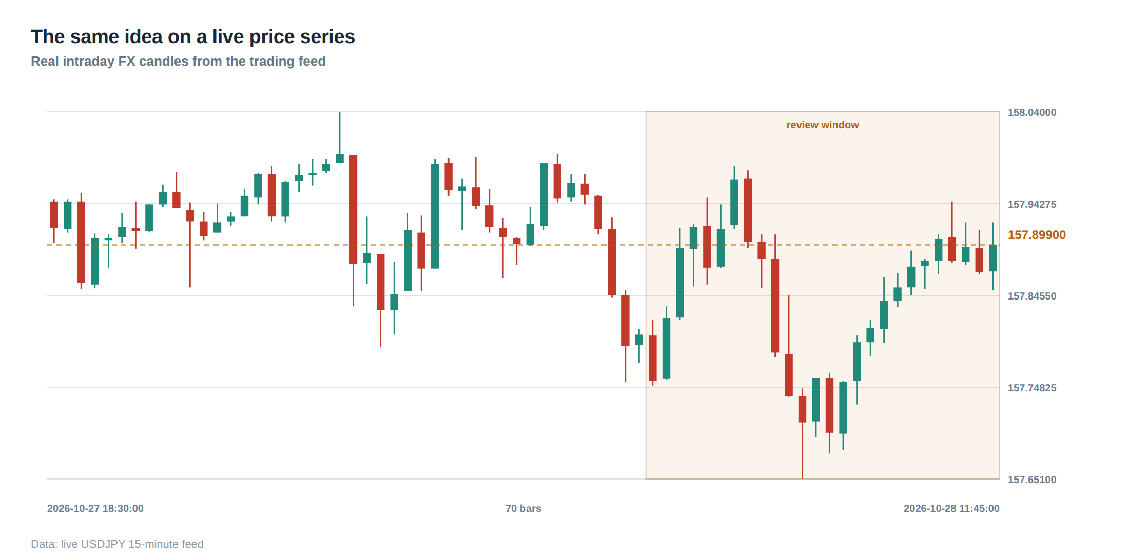
In a live environment the assumptions that underpin the statistical test can be violated abruptly. A sudden earnings surprise, a regulatory announcement or a macro‑shock can alter the fundamental drivers of the two securities, breaking the cointegration relationship overnight. The half‑life estimated on a rolling window may suddenly stretch to months, making the original convergence horizon unrealistic.

Execution also deviates from the idealised model. The queue‑based nature of modern electronic markets means that the order may sit in the book for several seconds, during which the spread can move against the trader. If the order is placed deep in the queue to minimise market impact, the adverse‑selection cost rises because the queue position is exposed to new information for longer. Conversely, aggressive routing to capture the spread quickly can increase slippage, especially in thinly traded instruments.

Another failure mode is data quality. Missing ticks, corporate actions that have not been correctly adjusted, or latency‑induced timestamp errors can produce artificial spikes in the spread. A wide z‑score generated by such an artefact will trigger a trade that appears to have a high expected profit but in reality carries no genuine convergence signal. Without robust data sanitisation the model can be repeatedly “tricked” by these anomalies, eroding capital over time.

The operating path, stage by stage

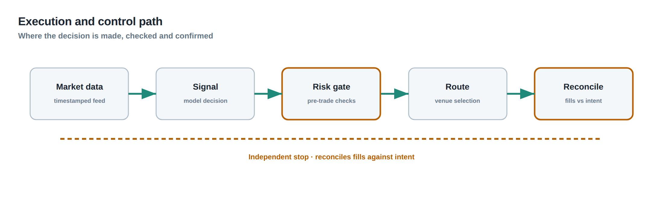
The trading system follows a deterministic pipeline. First, raw market data is ingested and normalised; corporate actions are applied and any out‑of‑range points are flagged. Second, the cointegration and half‑life diagnostics are recomputed on the refreshed window, and the common‑factor exposure is stripped from the raw spread. Third, the residual is standardised to produce a z‑score, which is then compared against both a price‑stop and a time‑stop horizon. Fourth, the cost model evaluates the net expected return; if it exceeds the desk’s risk‑adjusted threshold, the order size is calculated, respecting the exposure cap for the current regime. Fifth, the order is routed to the venue with a pre‑determined aggressiveness level, and a timer is started to enforce the time stop. Sixth, a real‑time monitor watches the live spread, queue position, and elapsed time; any breach of the stop conditions triggers an immediate unwind.

Each stage writes a diagnostic record to a central log, enabling post‑trade analysis and rapid identification of where a breakdown occurred. The flow is deliberately linear to avoid feedback loops that could amplify model risk when market conditions change faster than the system can adapt.

Controls that act before the damage

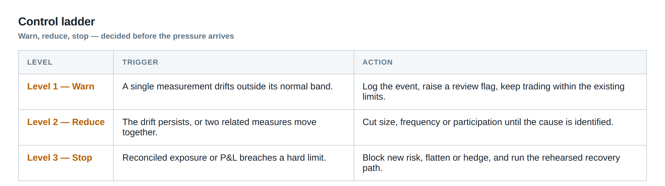
Preventative controls sit at the front‑end of the pipeline. A regime‑detection filter monitors macro‑indicators such as VIX, market‑wide liquidity metrics and sector‑specific news sentiment. When a shift is detected – for example a jump in VIX above 30 or a sudden drop in average daily volume for the pair – the system automatically tightens the z‑score threshold from 2.0 to 2.5 and reduces the exposure cap from 30 % to 10 % of capital.

A data‑integrity gate discards any price update that deviates more than five standard deviations from the last accepted value unless corroborated by at least two independent feeds. This guards against single‑source glitches that could otherwise generate a spurious wide spread.

A borrowing‑capacity monitor checks the desk’s current short‑sale inventory and the prevailing borrow rates. If the short leg’s borrow cost exceeds 0.8 % p.a., the algorithm flags the pair as “expensive to short” and either reduces the allocation or suspends trading on that pair until rates fall.

Finally, a “stop‑loss ladder” enforces layered exits: the first rung is the price stop (z‑score 4.0), the second rung is the time stop (20 days), and the third rung is a capital‑drawdown trigger (e.g., a 2 % loss on the pair’s cumulative P&L). Crossing any rung initiates a forced liquidation, preventing a small model error from snowballing into a large loss.

How to measure whether it is working

Performance measurement must separate true spread‑capture from the cost side‑effects. The primary metric is the “net convergence return”, defined as the realised profit after subtracting borrow, funding, turnover and execution costs, annualised on a per‑trade basis. A secondary metric is the “half‑life realised vs. expected” ratio; a ratio close to one indicates that the model’s reversion speed estimate remains valid.

Risk‑adjusted statistics such as the Sharpe ratio of the net returns, the maximum drawdown per pair, and the frequency of stop‑loss triggers provide insight into model‑risk exposure. A rising frequency of time‑stop exits, for instance, signals that the half‑life assumption is deteriorating.

The desk should also track the “model‑risk loss” – the portion of loss attributable to the spread failing to revert, isolated by stripping out the deterministic cost component. Comparing this figure across regimes helps decide whether to tighten thresholds or retire the pair altogether.

The portfolio view

At the portfolio level the statistical‑arbitrage book is treated as a collection of independent mean‑reversion bets, each with its own exposure cap and stop rules. Correlation analysis across the residual spreads ensures that the aggregate portfolio does not concentrate on a single hidden factor; a low‑rank factor model is applied to the net returns to confirm diversification.

Capital allocation is dynamic: when the overall model‑risk loss breaches a pre‑set budget (e.g., 0.5 % of total equity in a month), the system reduces the global exposure multiplier, effectively scaling down all active positions. Conversely, a period of low model‑risk loss and stable half‑lives permits a modest increase in the exposure caps, but never beyond the desk’s maximum leverage limit.

Liquidity monitoring is also essential. The aggregate turnover of the book should stay within the market’s capacity to absorb the trades without moving the spread materially. If the average daily turnover approaches a pre‑defined percentage of the average daily volume of the constituent securities, the system throttles new entry signals until the pressure eases.

By treating each pair as a micro‑risk and the collection as a macro‑risk, the desk can maintain a disciplined stance: statistical arbitrage remains a source of incremental return only while the underlying statistical relationships are demonstrably stationary and the cost structure remains favourable.

Will your current statistical‑arbitrage framework survive a sudden regime shift, or will model risk erode the edge you rely on?

About the research behind this lesson

The seminar frames electronic markets as price-time-priority queues. It separates queue value into spread capture versus adverse-selection cost and the option value of retaining a place in line.

Applied to this lesson: An order lifetime therefore cannot be based on elapsed time alone: the system must reassess whether its queue position, expected spread and adverse-selection risk still justify keeping the order alive.

Two live systems, one desk

PULSE-X — power-packed HFT: high-frequency momentum on XAUUSD and EURUSD. System details · Live account

NIC-X — ultra-low drawdown: displaced-print arbitrage for large capital. System details · Live account

Start now: leave your email and request a free trial — we will send the pricing, the connection route and the trial terms. Pricing

Live chat and updates: Telegram @xtrskhft

Source: High-Frequency Trading and Modern Market Microstructure

Educational content only. Trading leveraged products involves risk.